 BioPhysCode
This page describes an introductory lab exercise in which you will simulate and analyze a molecular dynamics simulation of a protein. This exercise follows the principles outlined in the pipeline tutorial, however students will need an instructor to set up a server for them. Students should receive a web address to begin.
Outline
- Starting with the factory
- 1. Analyze a protein simulation
- 1.1 Prepare metadata
- 1.2 Compute the protein RMSD
- 1.3 Download the trajectory
- 2. Simulating a new protein
- 2.1 Visit the simulation in the terminal
- 3. Hydrogen bonding
- 4. Principal components analysis
- Appendix: custom calculations
- Computing the RMSD “by hand”
- Hydrogen bonding walkthrough
Starting point: the “factory”
There are many different ways to create a molecular dynamics (MD) simulation. The Radhakrishnan lab typically uses the open-source GROMACS integrator to run the simulations because it is reliable, easy-to-use, and compatible with many different force-fields. Most scientific computation occurs with simple tools, namely a text editor and a terminal. GROMACS, and other integrators like NAMD and AMBER can be run at the terminal or one of many different graphical interfaces.
This lab exercise will cover the basics of generating and analyzing a protein simulation by using a piece of software developed by Ravi’s students called the “factory” which acts as a basic interface to the text files, binary executables, and command-line inputs required to run a simulation. Where possible, we will explain what the factory is doing at each step in the exercise for users who may wish to use these tools outside of the factory interface. Otherwise, users can generate and analyze data entirely in a web browser with the help of a Jupyter notebook. Each group will have access to their own project, running inside of an independent Docker container. We will perform all of the analysis in Python. The factory is designed to ensure that our research is standardized and replicable.
1 Analyze a protein simulation
Students have been given a web address to their own copy of the factory codes. We have also run a short 200ps simulation for you to analyze. Later you will generate your own simulations.
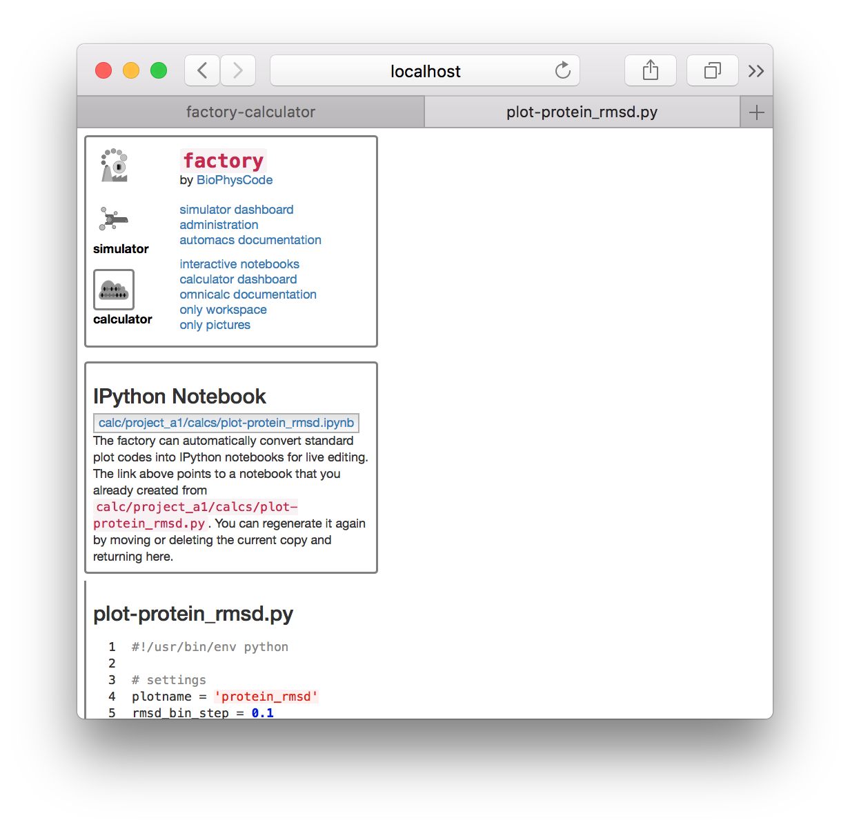
▶ Navigate to the factory website. The address will follow the pattern hostname.server.com:8000 where the number is the port. You will be asked for a username and password. The factory pages will often link to a Jupyter notebook server located on a different port.
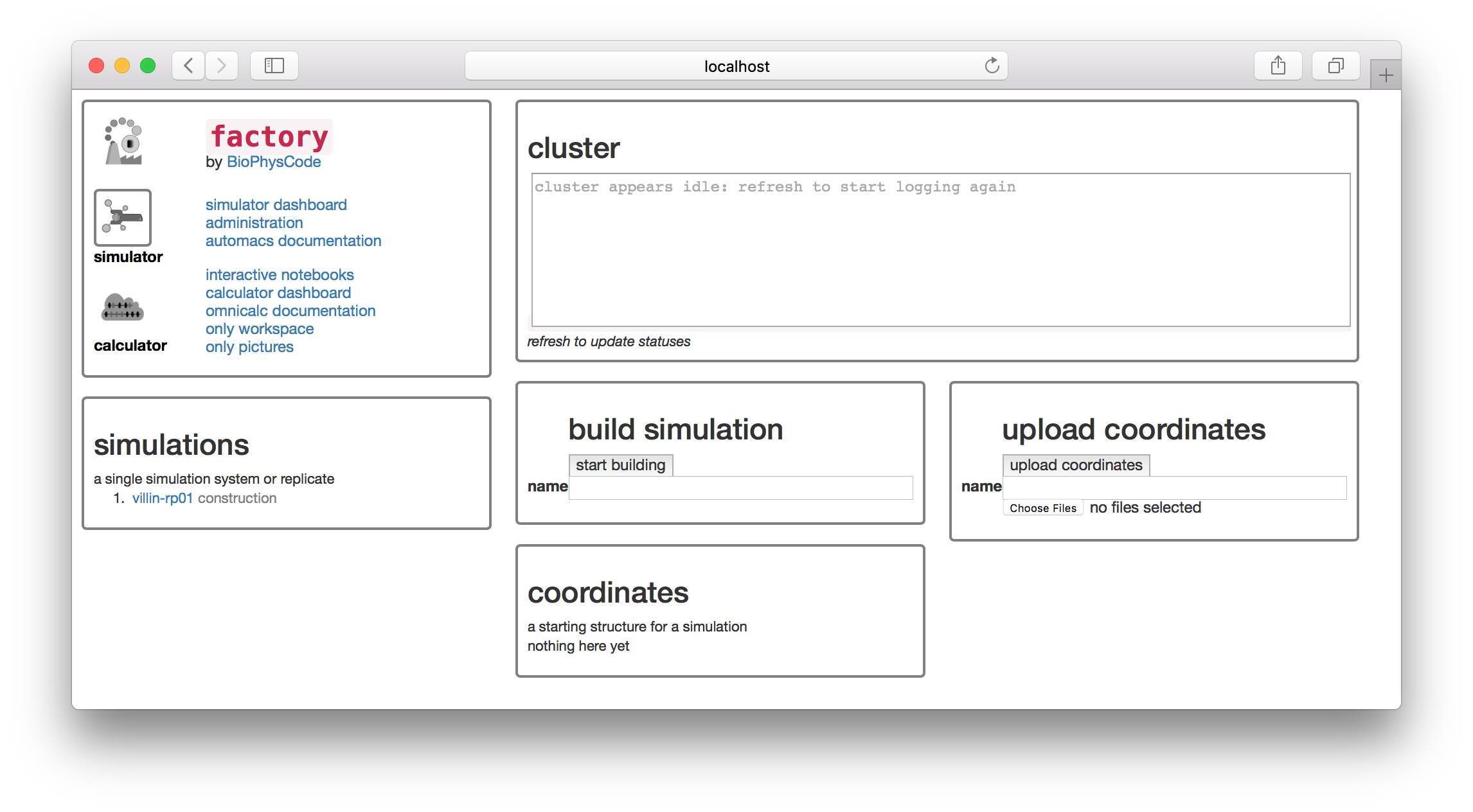
The factory has a “simulator” and “calculator” page, which you can access from icons on the navigation tile in the upper left. The navigation tile also contains a link to the “interactive notebooks” which will take you to the notebook server. This exercise is designed so that we can swiftly get our simulation data into a Jupyter/IPython notebook where it will be easy to analyze using standard tools.
You will find a simulation named villin-rp01 on the simulations list. In this section we will take the source data from this simulation and prepare a sample of the trajectory (a “slice”) that we can download and analyze. The factory will do this automatically when we run the first calculation. We can do this from the calculator page.
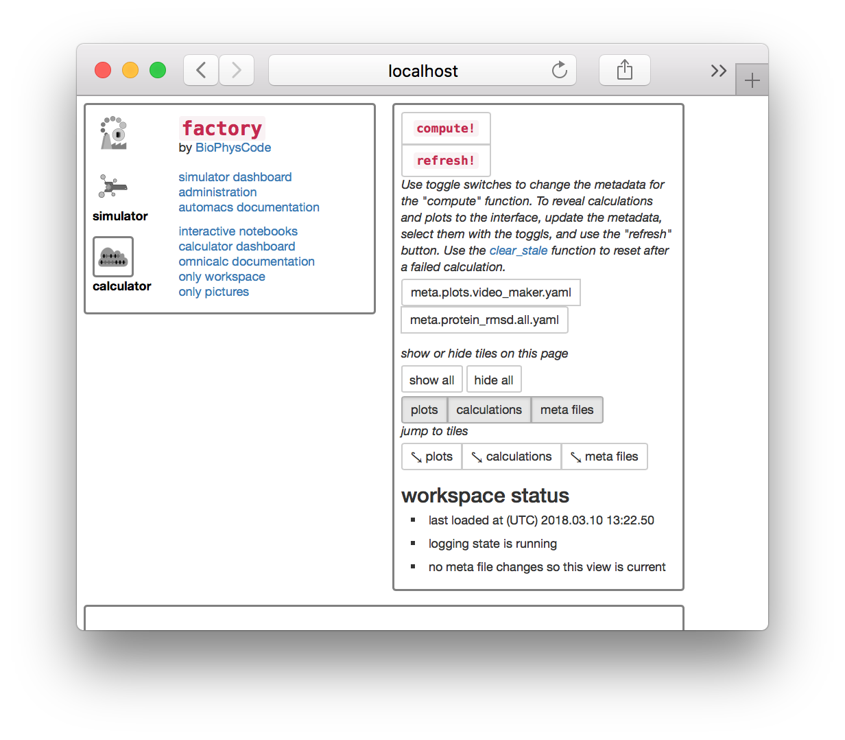
▶ Click the “calculator” button in the navigator tile to switch to the calculator page.
1.1 Prepare metadata
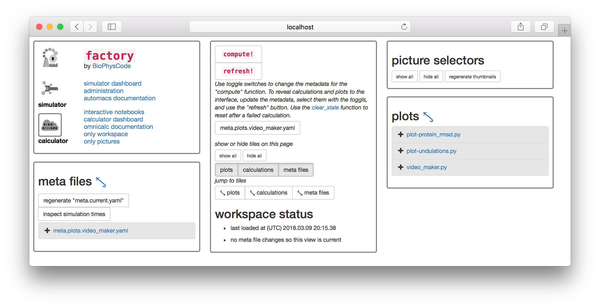
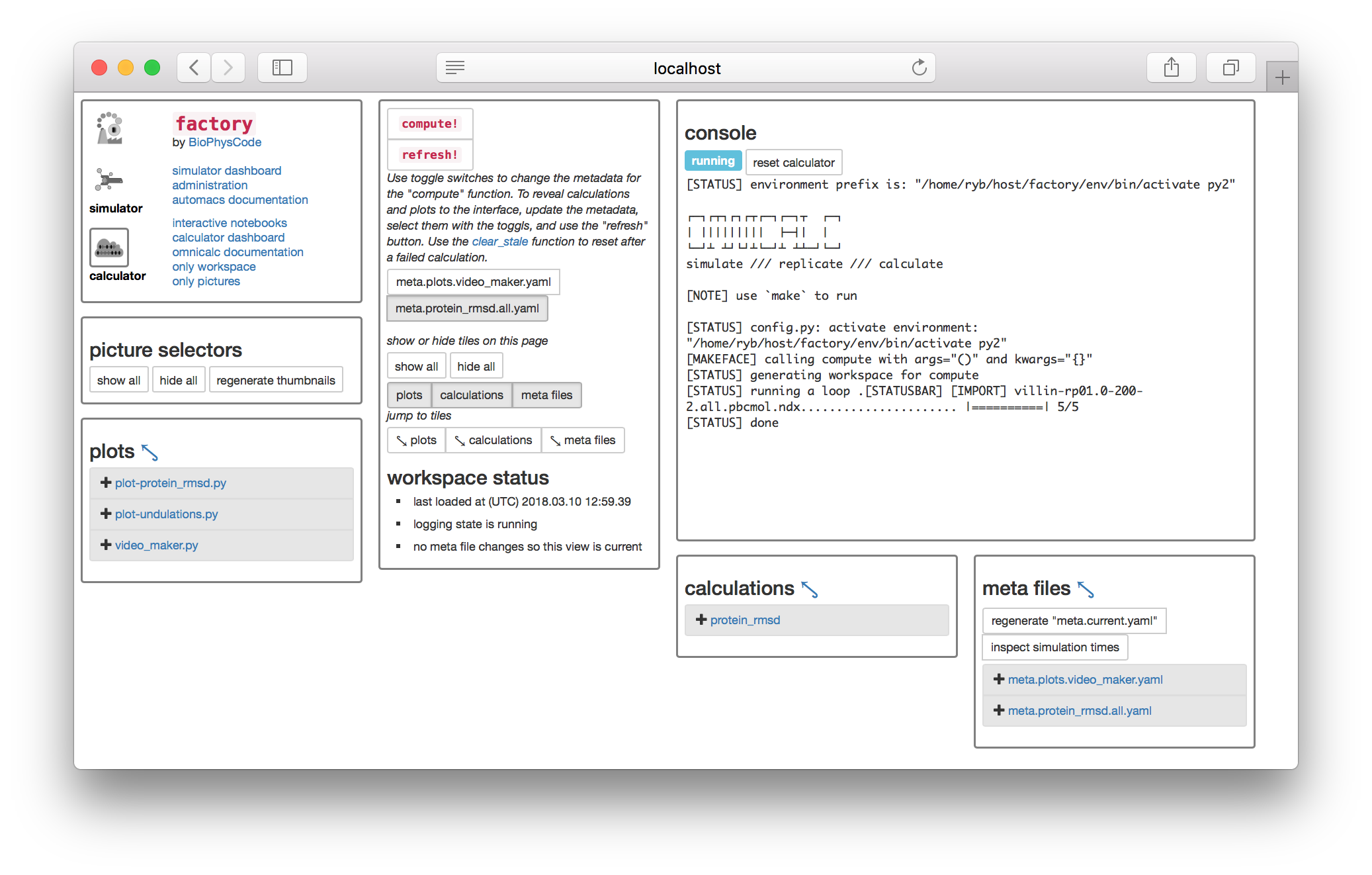
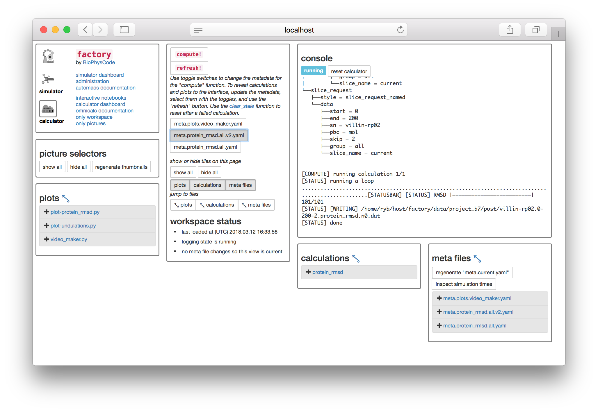
Most scientific computing happens at the command line or in a piece of software with a graphical interface with buttons and menus (e.g. VMD). The calculator is slightly different. We will first prepare a text file containing “metadata” that tells the calculator how to analyze the data, and then click the large compute! button to execute the instructions. There are toggle switches below the compute button that will let you select the metadata files. The image above has an extra file
The factory will automatically generate metadata for the most common calculation: the protein root-mean squared deviation (RMSD).
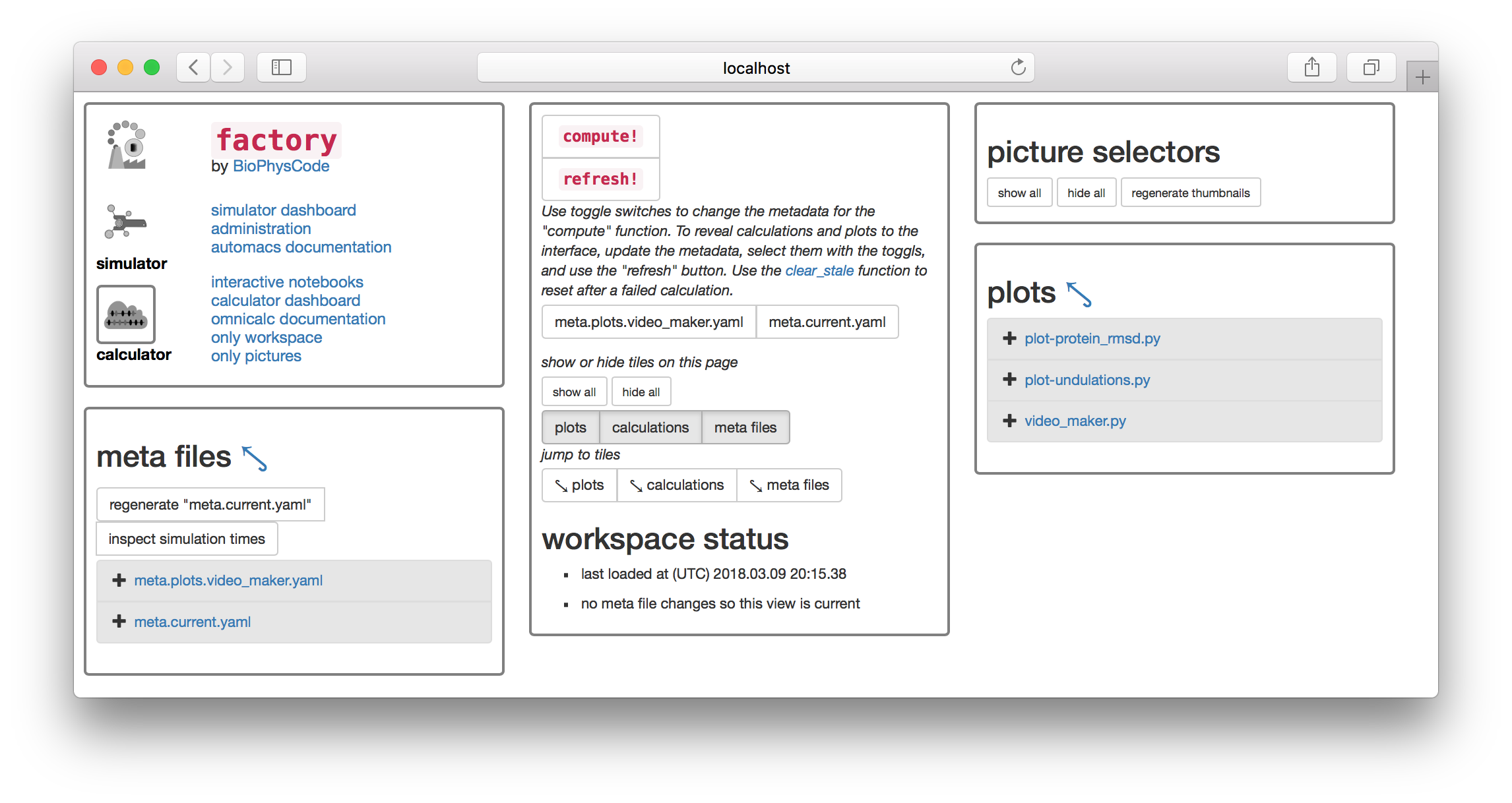
▶ Click the button titled regenerate "meta.current.yaml" which can be found on the “meta files” tile. This will cause the link meta.current.yaml to appear on the list below.
▶ Click the link and it will open the file in an editor in another browser tab.
This file is written in the YAML format which means that it is neatly organized by indents (some entries use braces to achieve the same effect). It includes three sections. The calculations section points to code that will analyze the simulation, the collections section has groups of simulations which can be analyzed together, and the slices section requests a slice of the simulation trajectory.
Before we continue, we will make a small change to the file. By default, it is set to sample only the coordinates necessary for the protein RMSD calculation, namely the “protein”. For later analysis we wish to use the entire simulation, including water and countions, in our trajectory slice.
▶ This means we need to change the word protein to all in several places. See the code below for the completed product.
- Change
group: proteintogroup: allin theprotein_rmsdentry of thecalculationssection. - Change the text
protein: proteintoall: allin thegroupsentry for the simulation (in this casevillin-rp01but later you may have a different simulation name or a list of simulations). - Lastly, change the
groups: proteintogroups: allin thecurrententry of thevillin-rp01entry in the slicessection.
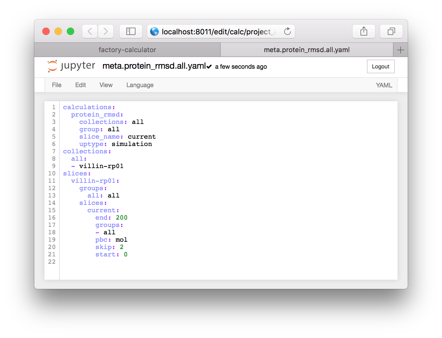
These changes will create the following text.
calculations:
protein_rmsd:
collections: all
group: all
slice_name: current
uptype: simulation
collections:
all:
- villin-rp01
slices:
villin-rp01:
groups:
all: all
slices:
current:
end: 200
groups:
- all
pbc: mol
skip: 2
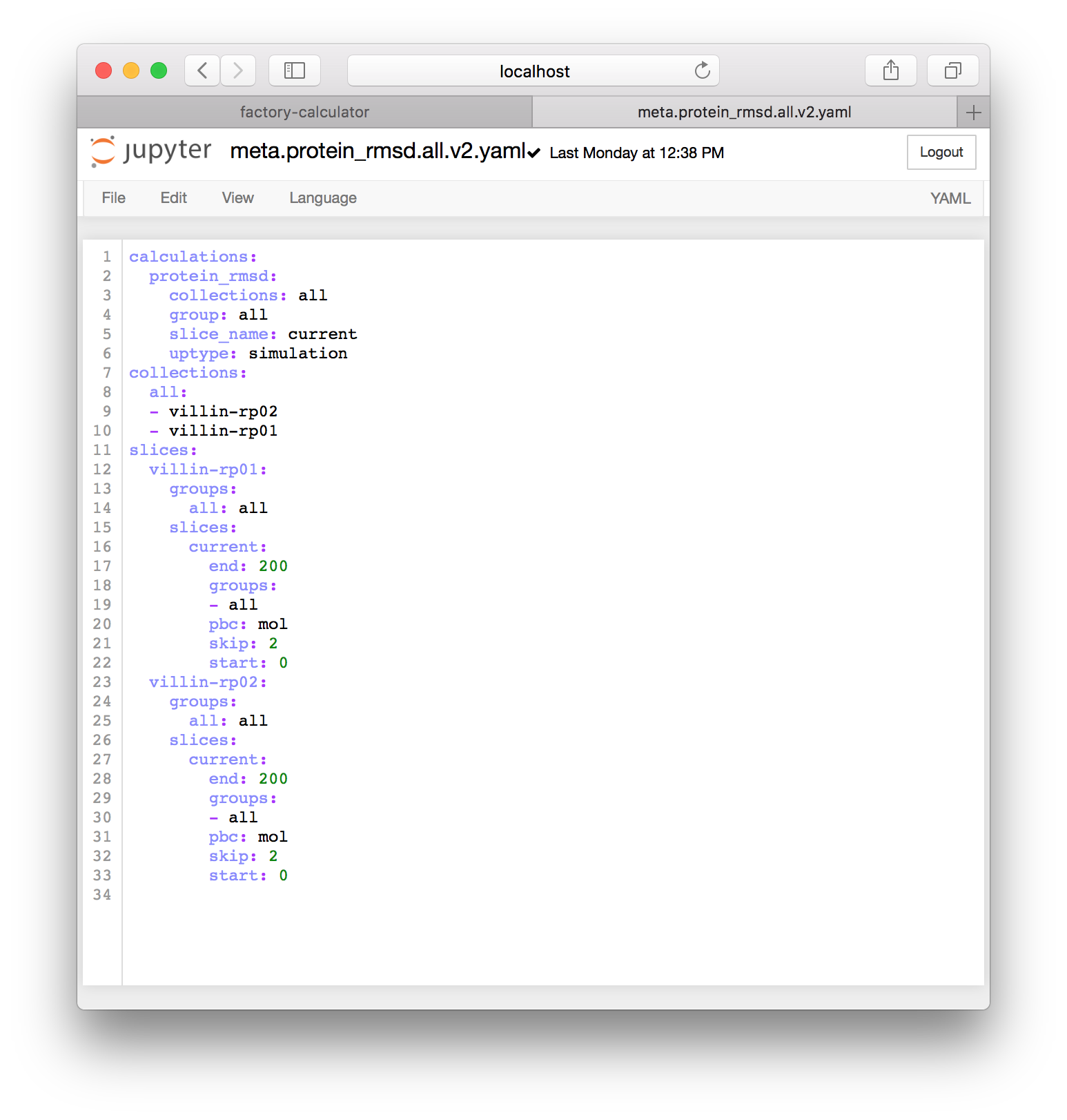
start: 0Each item in a YAML file is either a dictionary or a list. The text uses names to point from one object to another. It effectively tells the calculator to make a slice called current which will sample the trajectory from 0-200ps at a sampling rate (skip) of 2ps. The slice contains atoms from a group called all with an MDAnalysis selection text that is also all. MDAnalysis is the Python library which we use to read the simulation trajectories. Note that the selection commands for MDAnalysis, which we will use later, are very similar to those used in VMD.
▶ Click the name meta.current.yaml at the top of the editor and change it to meta.protein_rmsd.all.yaml to rename the file. When you have made these changes, your file should look like the one below.
Make sure you save the file with ctrl + s or the file menu. Note that you must click the text before using keyboard shortcuts otherwise the browser gets confused and will try to save the webpage instead.
1.2 Compute the protein RMSD
Now that we have prepared the correct metadata, we will compute the RMSD and receive a sampled trajectory as an added benefit.
▶ Return to the calculator page and click the toggle button named meta.protein_rmsd.all.yaml found underneath the compute! button. This selects the metadata you just created. Then click the compute! button. The console will appear with some text.
The compute button has (1) created a slice on disk and (2) calculated the protein RMSD of this data. Let’s view the calculation code.
▶ Toggle the meta.protein_rmsd.all.yaml again and click the refresh! button. This will reveal the calculations tile so you can click the link to the protein_rmsd code shown in the image above. The code will be displayed on a separate web page.
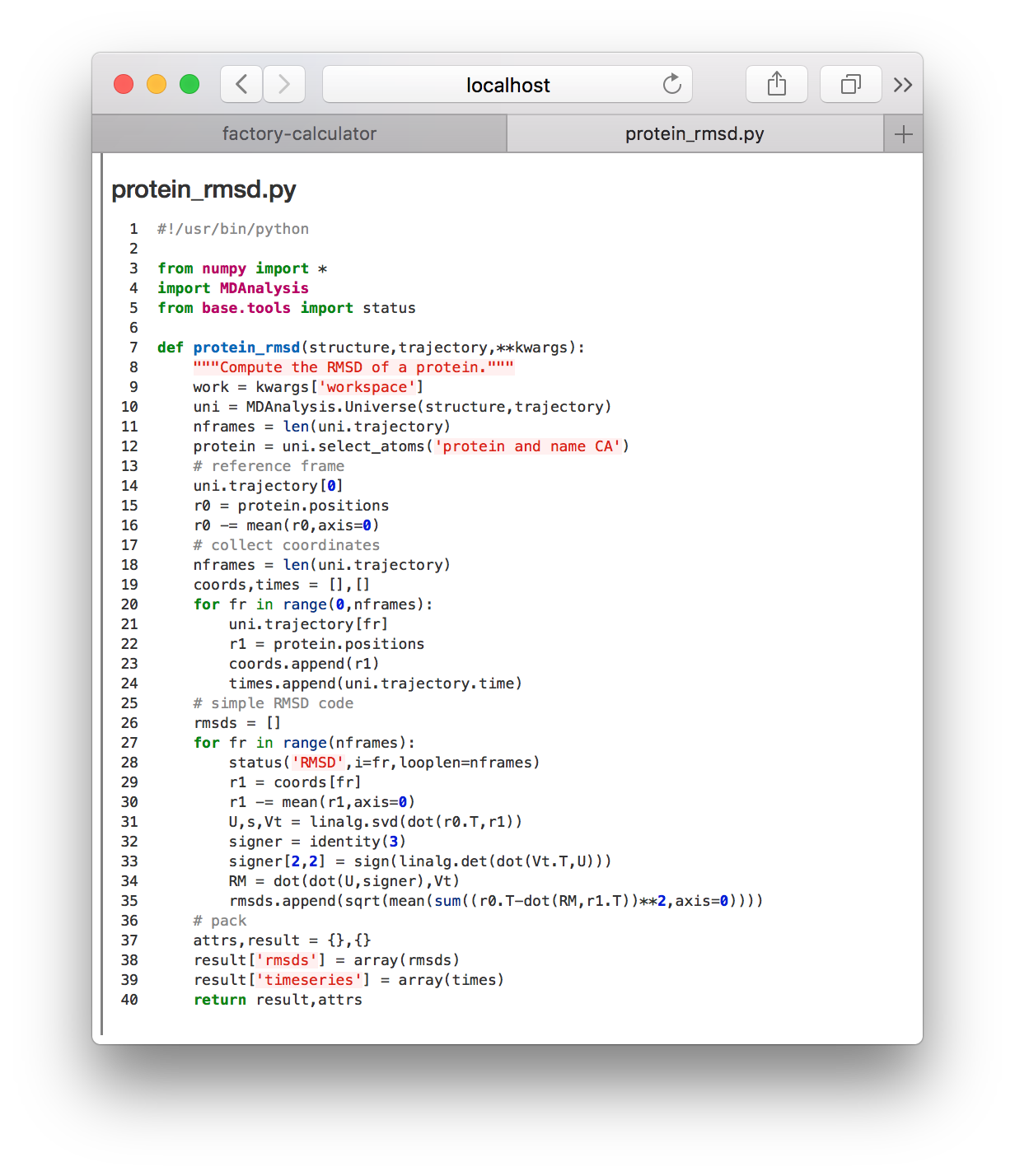
This code receives the simulation trajectory path, reads it with MDAnalysis, aligns the protein, and then saves the timeseries for the RMSD relative to the first frame. Later we will perform this analysis ourselves, in a Python notebook. For now, we will visualize the results of this calculation in a separate notebook dedicated to ploting the result.
▶ Return to the calculator page, which might be open in another tab. Click the plot-protein_rmsd.py link in the plots tile. This will take you to a page with the visualization code.
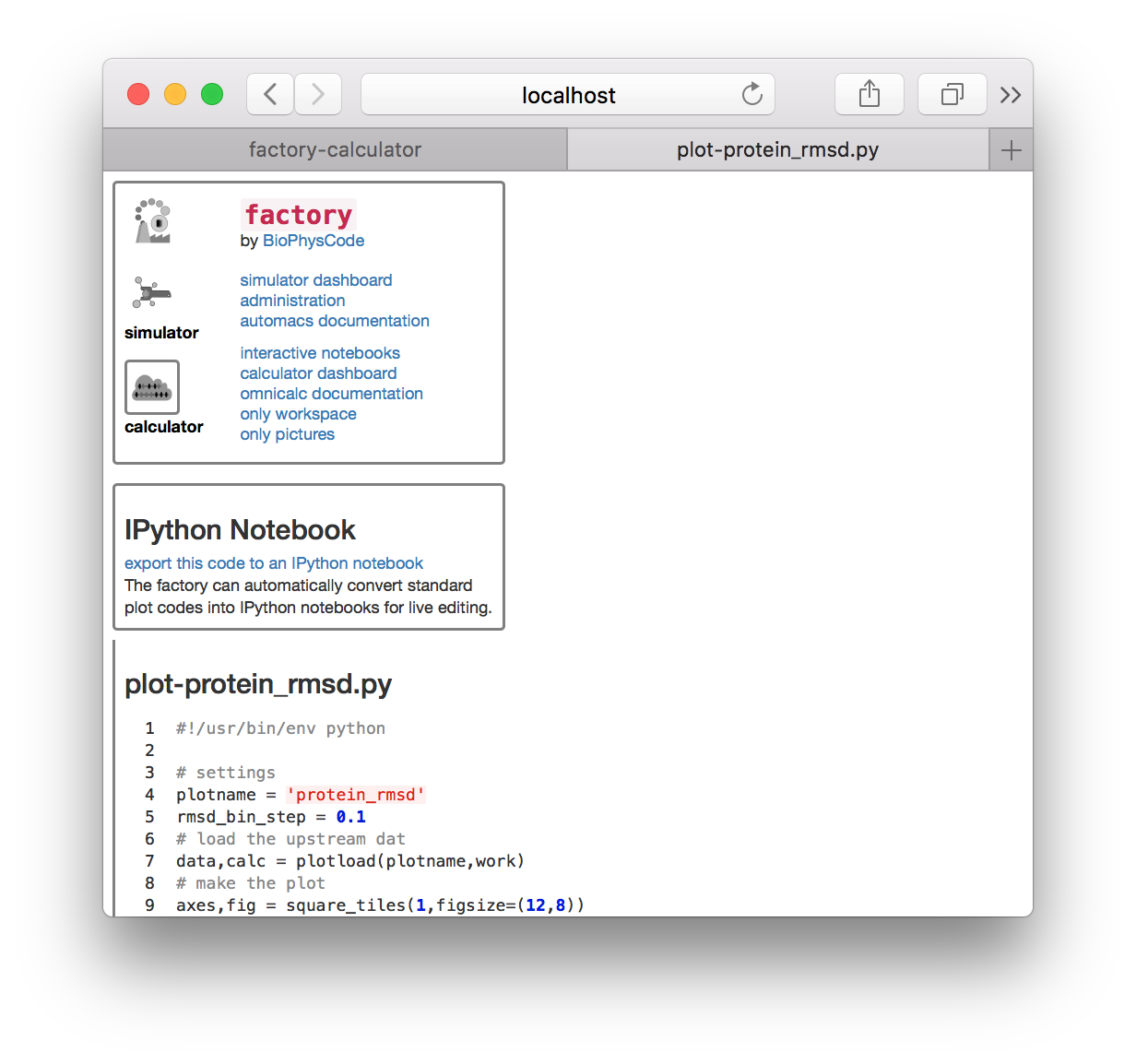
▶ Click the link “export this code to an IPython notebook” to make an interactive notebook. A button will appear when the page refreshes. Click the button to open the notebook.
The visualization code has been automatically added to an interactive Jupyter notebook so we can analyze and plot the results. The notebook is composed of cells which you can select (which creates a green border) and execute by typing shift + enter.
▶ Execute each of the cells in the notebook by clicking on them and typing shift + enter. You should see a protein RMSD plot below.
▶ If your code does not plot a legend, add ax.legend() directly above the comment that says “save the figure”. If you have multiple simulations, this will help to distinguish the data for multiple simulations if you run more than one.
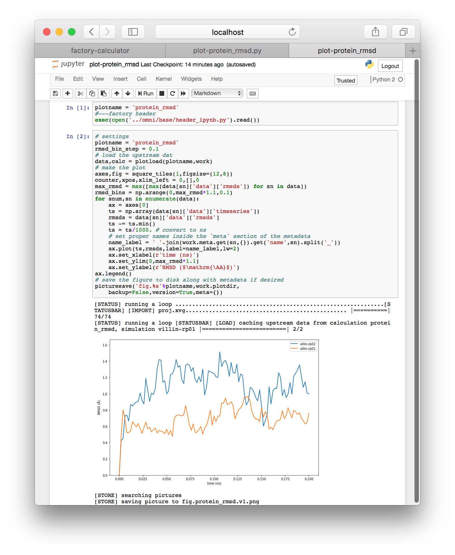
The Jupyter notebook resembles MatLab and Mathematica and has a wide body of documentation if you want to learn more. You can make new cells by typing “b” for below or “a” for above when you have selected a cell. You can also type the names of variables to view them in an output cell. The tag on the left of each cell will change from In [ ] to In [1] when it is finished. An asterisk tells you that the code is still running. Later we will develop our analysis in this environment, but the protein RMSD plot above should be automatic.
1.3 Download the trajectory
Now that we have completed one piece of the analysis, we can download the trajectory slice and visualize it in VMD. So far, we have used the factory website served from e.g. hostname.server.com:8000 however several links have taken us to the Jupyter notebook server, which is served on a different port e.g. hostname.server.com:8001. For security reasons, you can only access Jupyter from a link on the factory page.
▶ Click on the “interactive notebooks” link next to the calculator icon on the upper left tile in the factory. This link is the best way to get to the notebook server.
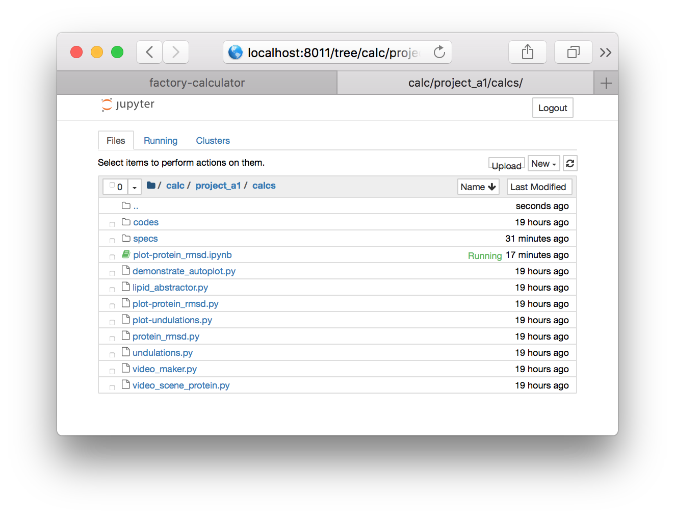
▶ Click the folder icon to the left of calc / project_a1 / calcs to navigate to the root directory. Note that your project name may be different.
▶ Using the folder links, navigate from the root directory to data/project_a1/post but be sure to use the project name associated with your group e.g. protein_b3. This will provide a listing of the trajectory files.
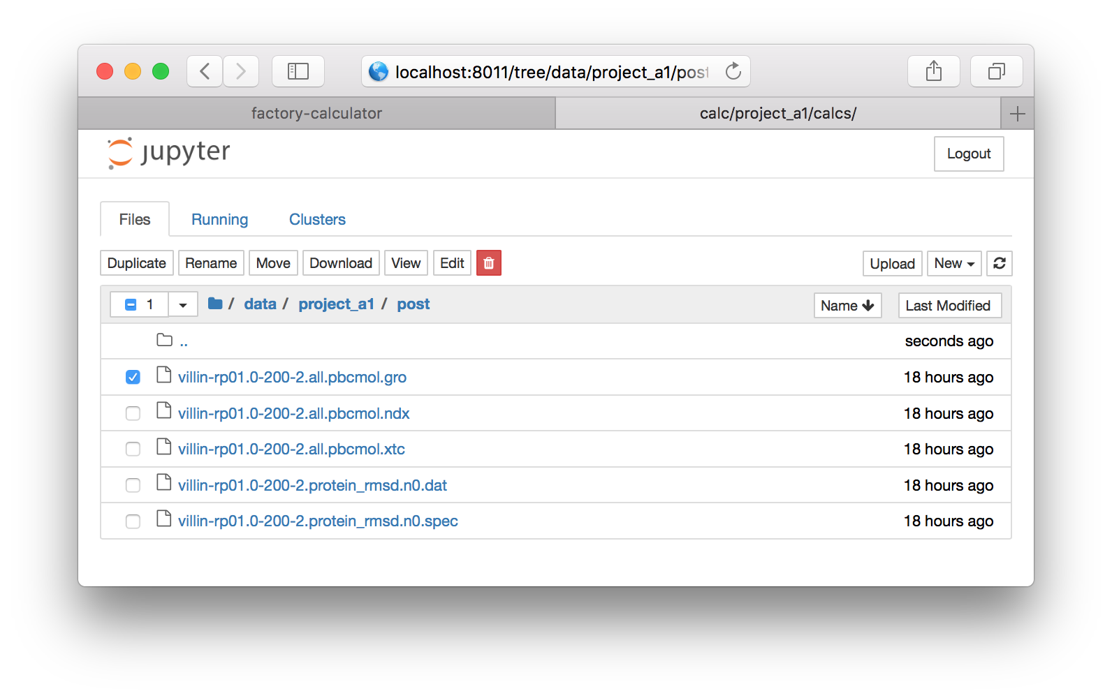
▶ Click the check box next to the file called villin-rp01.0-200-2.all.pbcmol.gro (see the image above) and click the download button on the bar above it. Save the file to your home directory. Repeat this with the XTC file called villin-rp01.0-200-2.all.pbcmol.gro. Note that you cannot download two files at once, so you have to uncheck the first file to download the second.
These files can be opened inside VMD to view the simulation. VMD treats the GRO file just like a PDB, while the XTC file is a binary file that must be opened. The factory has treated the periodic boundary conditions in the simulations so that the molecules do not “break” across the periodic boundary of the simulation when they move away from the center of the box. You can repeat the protein RMSD calculation in VMD, but it is also useful to see the structure of the protein.
2 Simulating a new protein
In the previous sections you have analyzed preexisting simulation data. In this section we will use the “simulator” to make another replicate. You can use this method to simulate any protein structure available on the protein data bank (PDB) as long as the structure is complete.
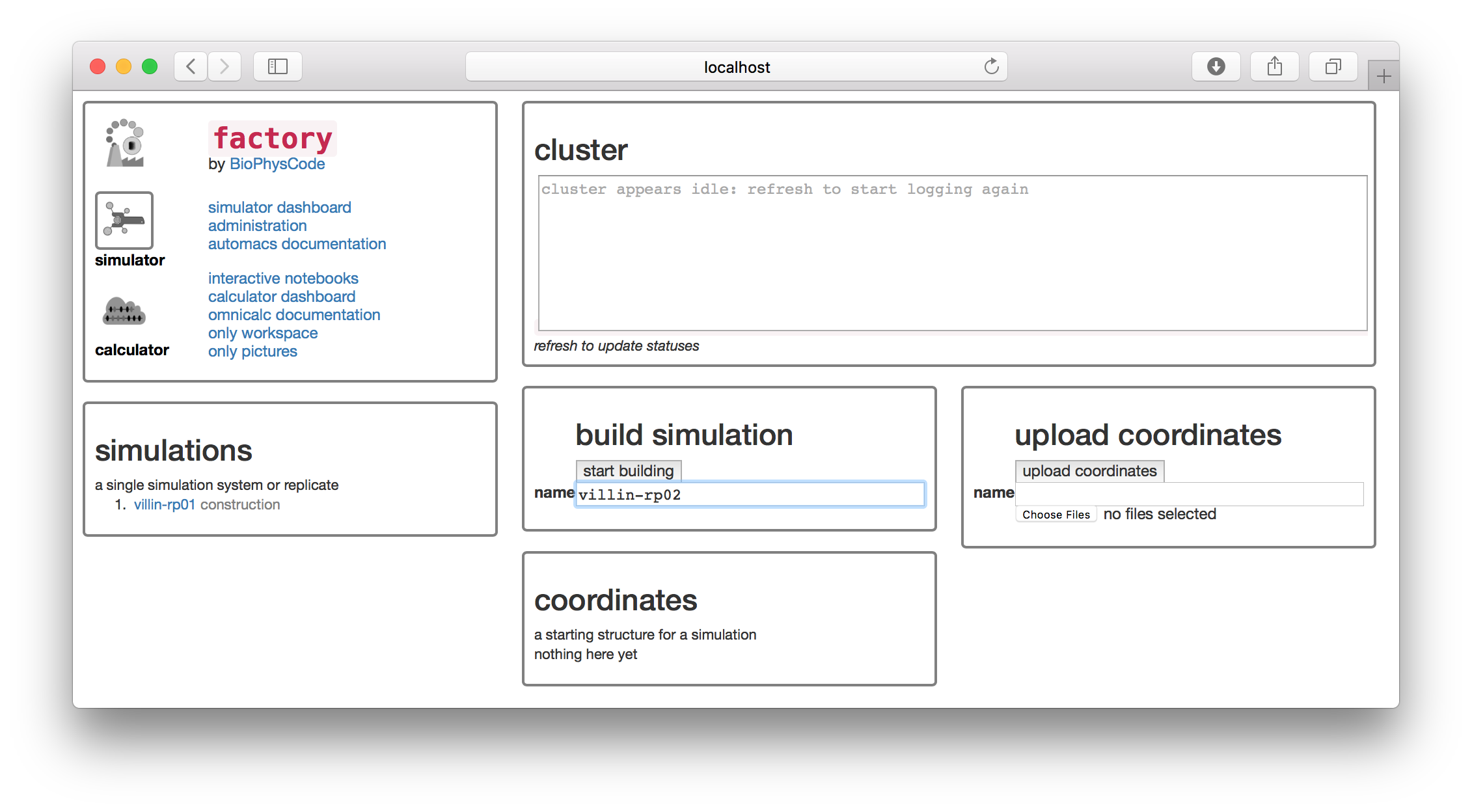
▶ Navigate to the “simulator” page on the factory using the icon in the upper left tile.
For this example, we will simulate one of the smallest, fastest-folding protein domains called the villin headpiece. In a subsequent exercise, we will also show you how to use custom targets, but for now we will draw on PDB to supply the starting structure for the simulation. We will name the simulation villin-rp02 since the simulation we analyzed in the previous section was the first replicate, villin-rp01. It is always a good idea to keep track of these names in a lab notebook.
▶ Type the name villin-rp02 in the text box in the “build simulation” tile.
The factory interface runs terminal commands in the background to generate the simulation on disk. For the remainder of the tutorial we will explain which commands it is running so that you know how these text-based tools work. You won’t need to run the commands yourself, unless you wish to reproduce the simulation at the linux terminal. Building the simulation is equivalent to the following command, which creates a new folder with the name of your simulation.
git clone http://github.com/biophyscode/automacs villin-rp02▶ Click the “start building” button.
The next page asks you to choose a “kickstarter” which adds codes to your simulation.
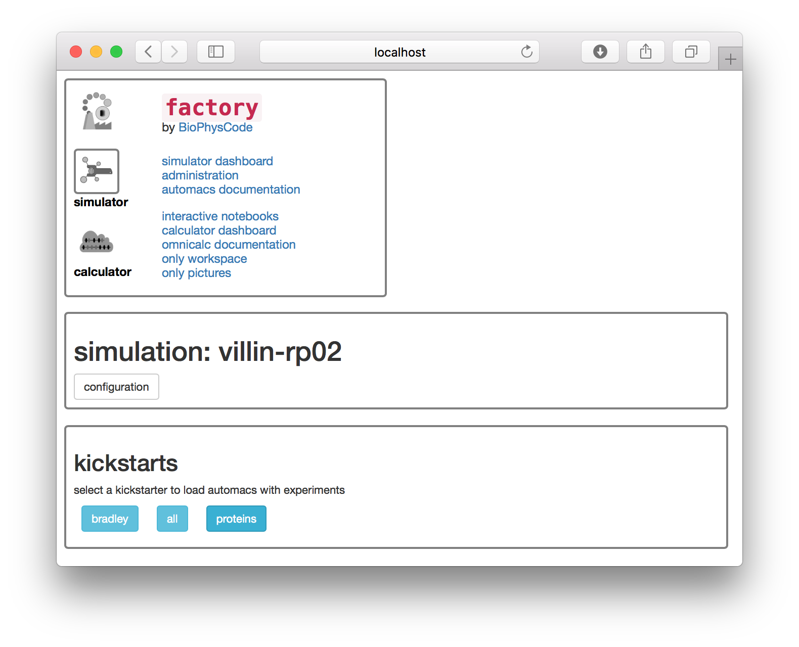
▶ Select the proteins kickstarter.
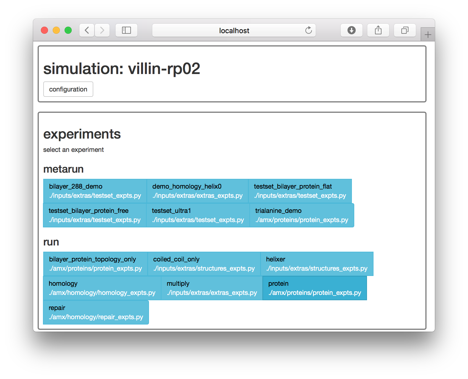
The factory has run the following commands on disk to prepare the protein simulation.
cd lyzosyme-rp01
make setup proteins
▶ On the web interface, the next page supplies a list of simulation “experiments”. Choose the protein experiment. Selecting this experiment is equivalent to the make prep protein terminal command.
The next page has a set of options for running this experiment.
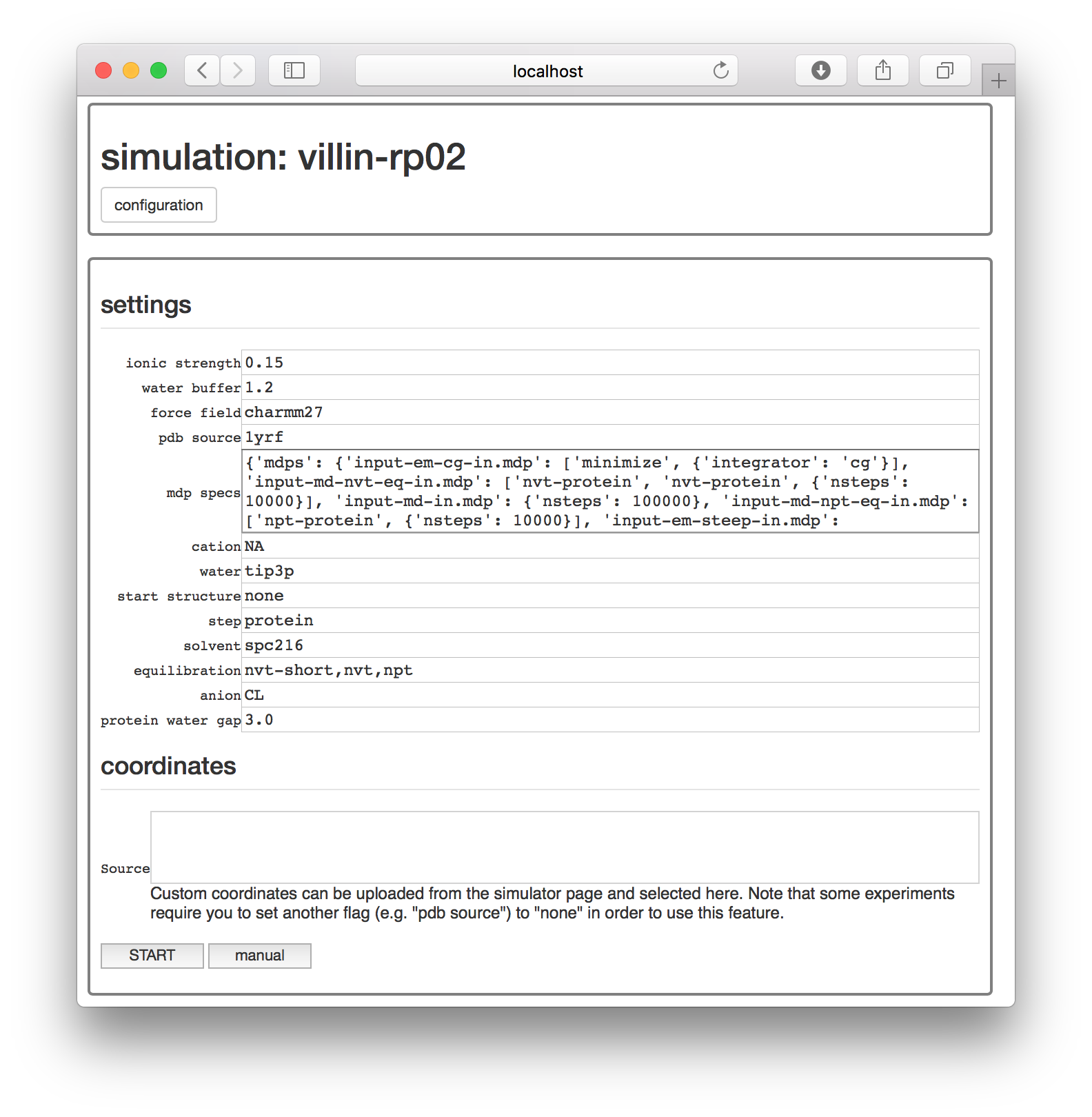
At this point, you could simply choose a protein databank structure by a four-character code, add it to the pdb source field, and run the simulation with the start button. However, for this exercise, we will take a closer look at the simulation by clicking the manual button, which generates an interactive notebook on a separate page.
▶ Click the manual button. The next page has an interactive script button.
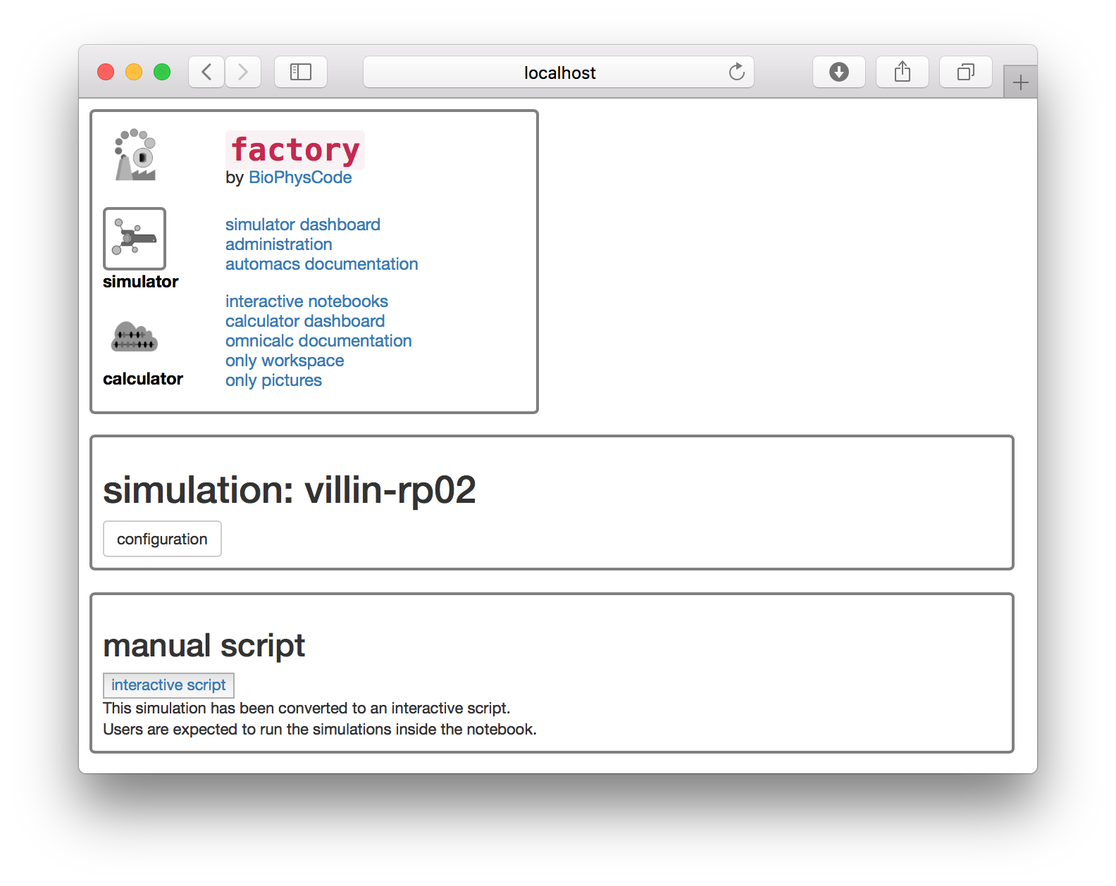
▶ Click the interactive script button to open the simulation notebook.
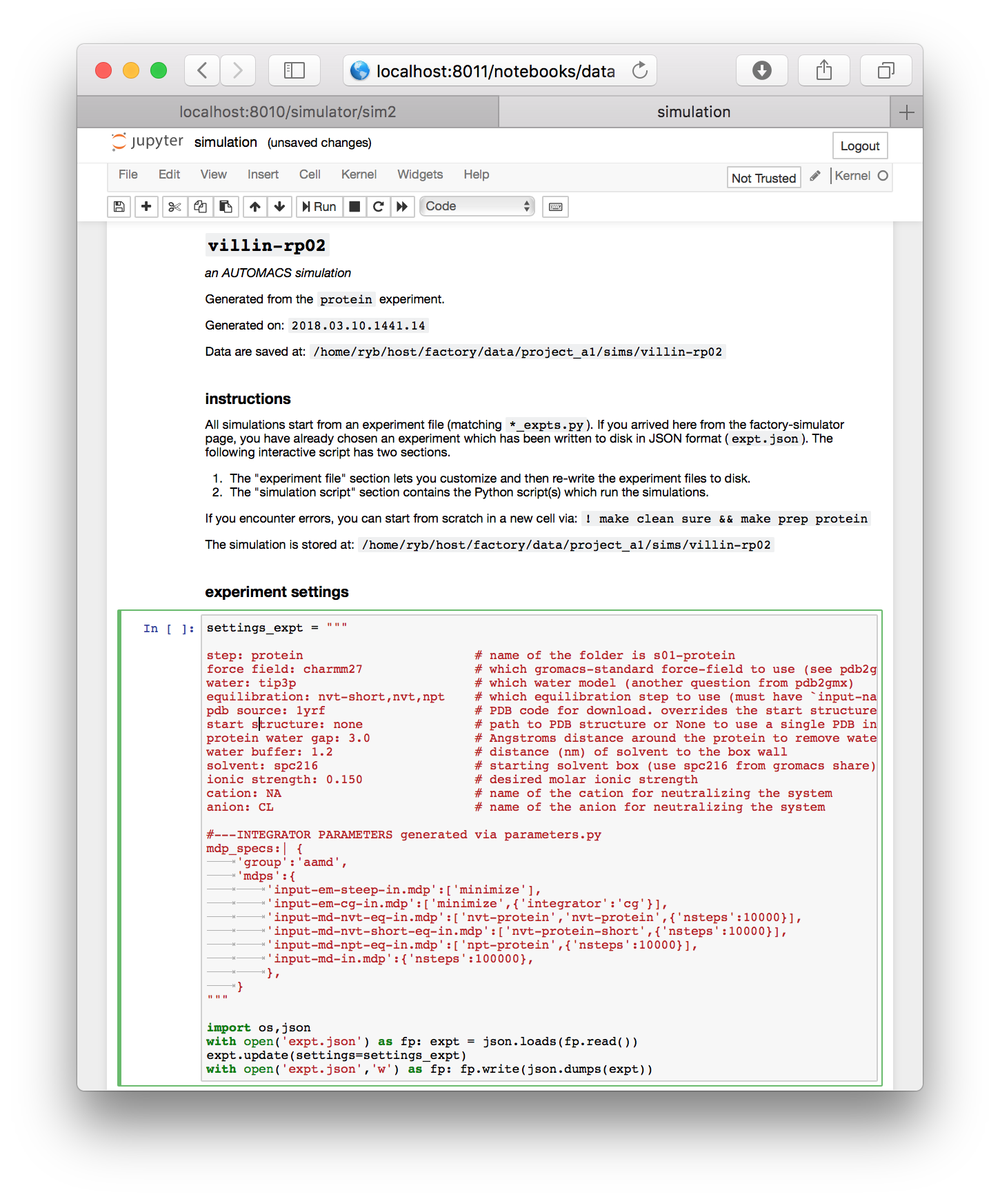
The simulation notebook begins with a “settings” block which is mostly text. You can change various features of the simulation here, including the chemistry of the counterions (cation and anion), the size of the simulation box (water buffer), and most importantly, the identity of the starting structure (pdb source).
For this demonstration, make sure the starting structure in the pdb source field is set to 1yrf. This is the PDB structure for the villin headpiece. In a later assignment, we will analyze a larger protein called lysozyme. Both structures are found on the protein databank (PDB) and can be accessed by their four-letter codes.
The protein experiment we will run in a moment consists almost entirely of GROMACS commands which mimic the excellent lysozyme tutotrial created by Justin Lemkul. This procedure takes the PDB coordinates as a starting point. The factory codes will automatically download the structure for you and feed it into the GROMACS pdb2gmx utility, which turns the coordinates and chemistry into a molecular dynamics “topology” containing information about the connectivity. It does this by following instructions given by the force field, which is specified in the settings block. For this example, we are using the charmm27 force field.
Note after this exercise, you are free to repeat this method for a different protein. To run a simulation of a different protein, first select the right PDB code. If the structure on the PDB requires no editing, then you can simply replace the pdb source field with the right code. For example, to simulate lysozyme you should change the field from 1yrf (a villin structure) to 1aki (a lysozyme structure).
Development note: we will add instructions for custom PDBs shortly.
▶ Once you have reviewed the settings, click the cell (the border will turn green) and execute the cell by pressing shift + enter. This will write the settings to disk.
If you encounter an error you may wish to start over. This requires two steps. First, use the kernel menu at the top to “Restart & Clear Output” which will reset the notebook. Second, make a new cell (you can use the “a” key or the “insert” menu) with the following contents: ! make clean sure && make prep protein. If you run this cell, it issues a terminal command that erases your data and resets the simulation.
The factory code is written entirely in Python, and most features can be used directly in the Jupyter notebook.
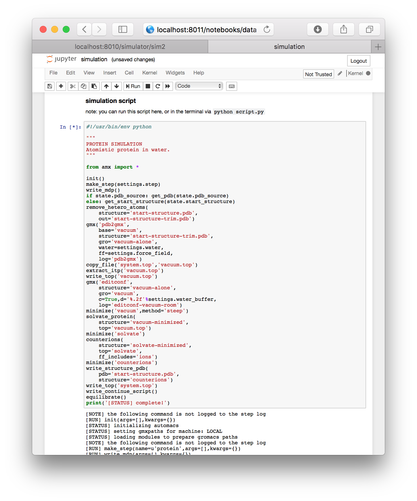
Once you have selected the 1yrf starting structure and executed the first cell, its tag will change from In [ ] to In [1] indicating that it is complete. The end of the cell contains a few lines of Python which writes the settings to a factory-specific input file called expt.json. The simulation itself is executed by a simple Python script which has been written to the next cell. You can see commands like solvate and equilibrate which we will discuss later.
▶ Run the final cell, containing the script. Note that this is identical to running python script.py from the simulation folder.
While the simulation is running, it will print a log underneath.
Running a simulation remotely. Users who wish to leave the browser while their simulation runs are welcome to do so. First, save the notebook (via ctrl+s) and then close the tab in your browser. Jupyter will ask if you are sure that you want to leave the browser. You are free to leave the page. If you return in Firefox, an hourglass icon will indicate whether or not your simulation is still running. Other browsers lack this feature, but you can always check your simulation using the terminal according to the instructions in the next section.
2.1 Visit the simulation in the terminal
The following section is optional. You can wait at the main factory (simulator) page until the simulation is complete (it will automatically update) or you can visit the in-progress simulation using the instructions in this section. We include this documentation for users who want to see how GROMACS is generating log files on disk.
While the simulation runs, you have the option to log in to the workstation to view the log files from the browser. Note that you should not use the ssh program to log in directly. For technical reasons, it is easier to use the browser we have provided in the browser.
▶ Open the link to the “shell” supplied for this lab on a separate port e.g. hostname.server.com:8003. For this tutorial, the port number should be two above the one that you use to access the factory. For example, if your factory is located at famous.scientist.school.edu:8020 then your shell can be found at famous.scientist.school.edu:8022.
After you supply a password you will see a linux shell or terminal. You can run ls to see the current folders, which should include host. Use the cd command to change directories to your simulation folder via cd host/factory/data/project_a1/sims/villin-rp02 (replace the name project_a1 or the simulation name villin-rp02 if you have a different project or simulation name). Then run tail s01-protein/s01-protein.log to monitor the simulation progress.
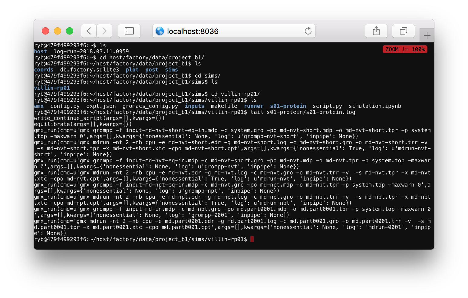
The log file tells you what the code is doing. Most of the items in this file start with gmx_run which is a Python function that runs a command at the terminal. One of the arguments to this function tells you the text of the command. For example, the final command is gmx mdrun -nt 2 -nb cpu ..., indicating that the program is running the mdrun binary to run the simulation. This line also specifies a log file, which you can view by running tail s01-protein/log-mdrun-0001. When the simulation is complete, you can see a benchmark which tells us how many nanoseconds have elapsed.
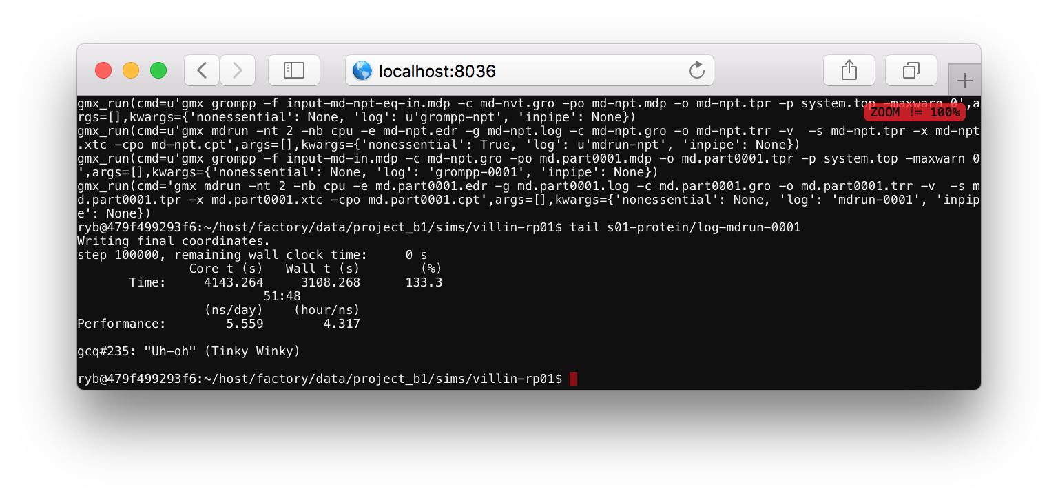
The simulation should only take a few minutes to complete. We recommend that you keep the simulation notebook open until it prints complete! to the output cell. The replicate that we have made in this exercise, called villin-rp02 can be analyzed in the same way we analyzed the first replicate, villin-rp01 in the beginning.
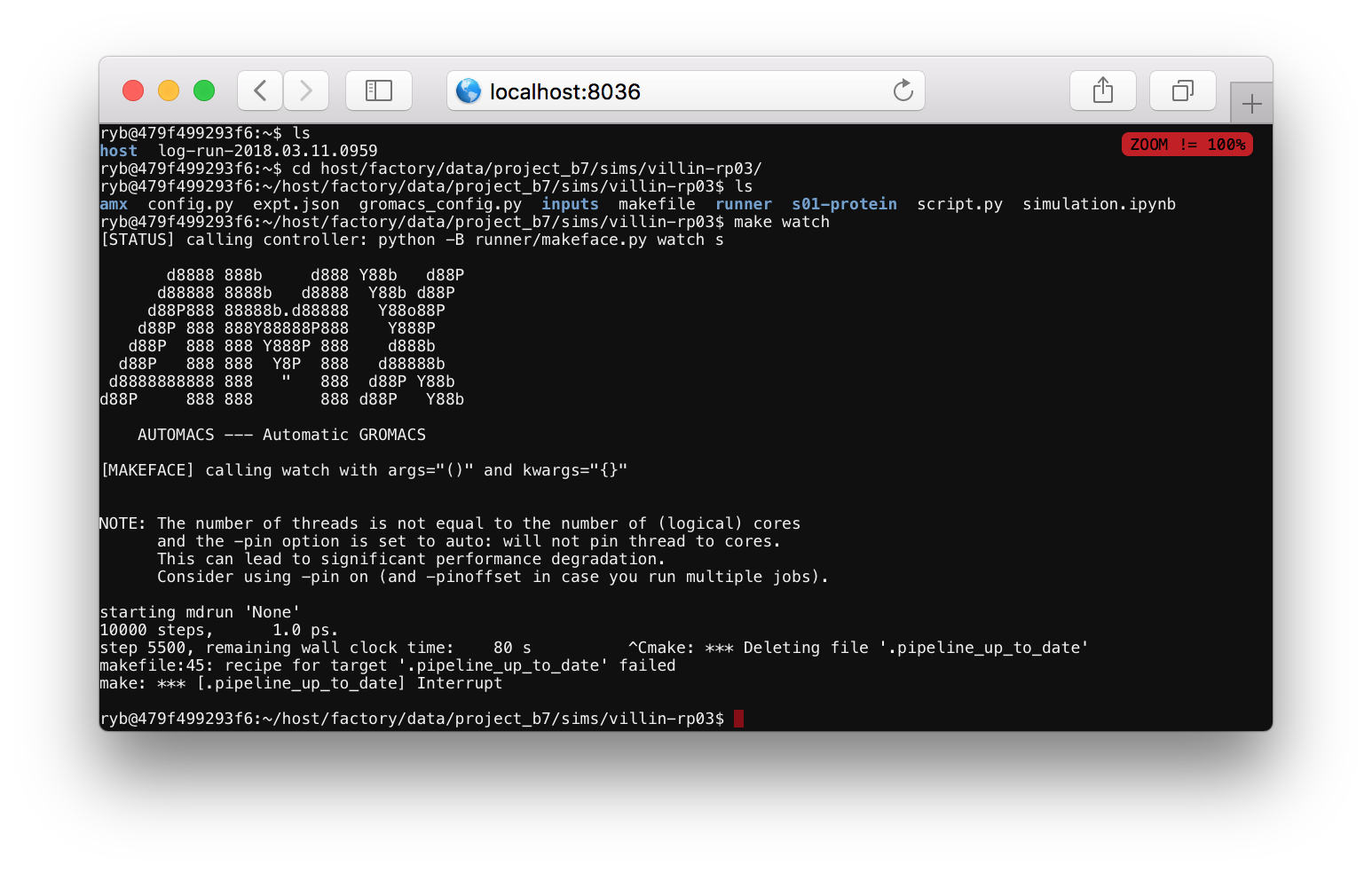
Checking up on a simulation. Users who start a simulation in a Jupyter notebook can check that their simulation is still running by navigating to the correct folder, for example host/factory/data/project_b1/sims/villin-rp01/. If you run make watch it will show you the last relevant log file. If it says that it has written the final coordinates, then your simulation is complete. Use ctrl+c to exit the make watch command.
Continuing a simulation. This step is optional. If you want to extend your simulation, change directories to the main (only) step by running cd s01-protein. Then, run ./script-continue.sh for a while. Use ctrl+c once it has run for a while to cancel it. Please do not let your simulation run indefinitely. It will run for 24 hours if you leave it unattended. Using this script will add more time to your trajectory. In a typical research project, we would send the simulation to a high-performance platform to accrue more time.
3 Hydrogen bonding
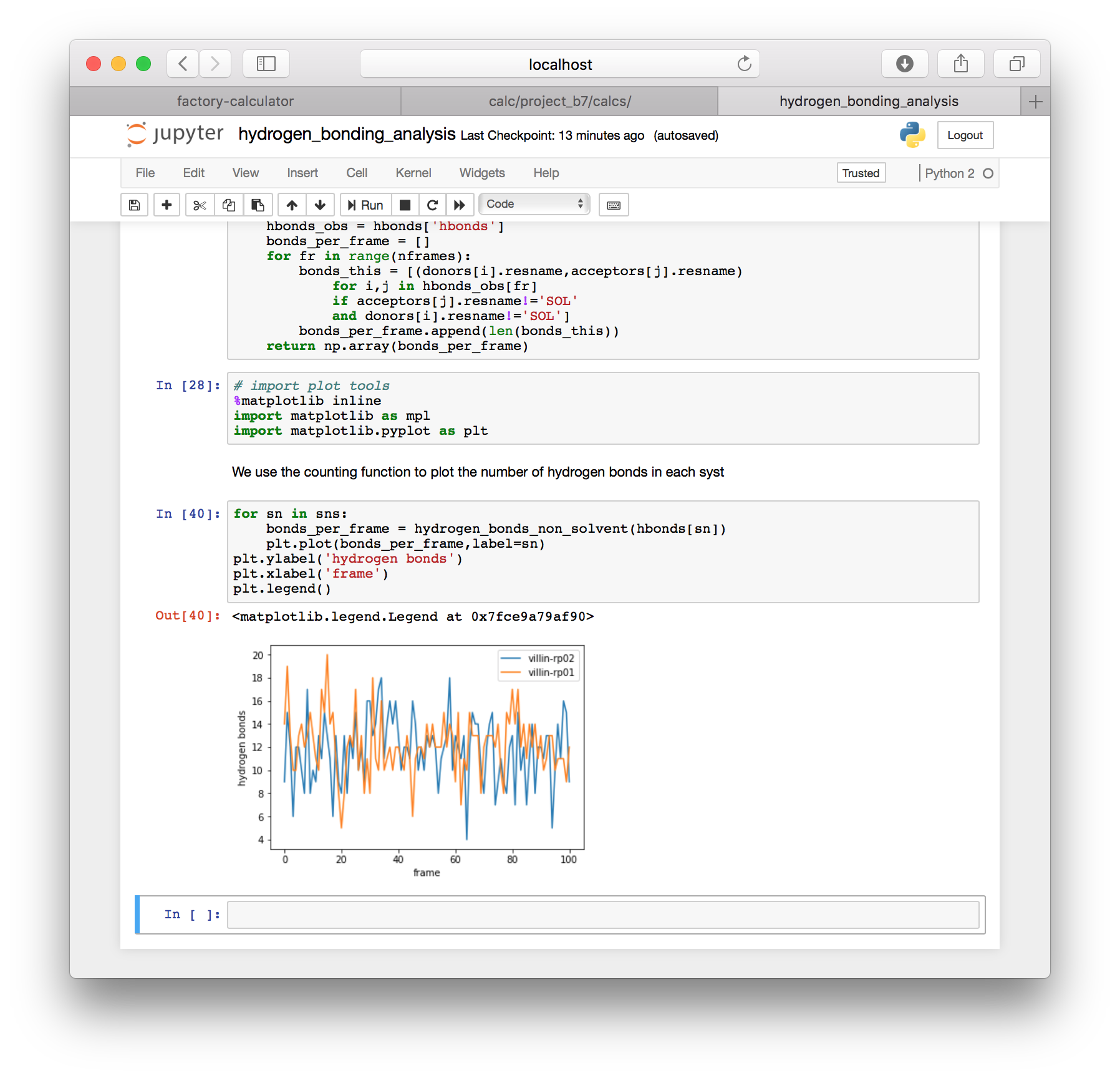
So far, you have learned how to use the automatic protein_rmsd code to copute the protein structural changes in a pre-made villin-rp01 simulation in the first section and then you learned how to start your own protein simulation. In this section we will tabulate the protein-protein hydrogen bonding in our system. This analysis will produce a list of each hydrogen bond found in each frame of your simulation trajectory. At the end we will make a plot of the number of bonds over time, however you can use the bond list to learn more about specific bonds.
▶ Go to the calculator page and click the “interactive notebooks” link. You should see a notebook called hydrogen_bond_analysis.ipynb in the list of files.
This script uses MDAnalysis to read in each simulation trajectory, searches for hydrogen bond donors and acceptors, and then uses a K-D Tree to find pairs which are close to each other. Once it does, it filters these by configurations that have a high (i.e. nearly straight) angle. We expect these bonds to be strong, and hence relevant to the dynamics of the protein’s shape.
▶ Execute each cell of the notebook by using shift + enter. If you encounter errors you may need to use the stop button at the top, or restart the kernel using the menus.
The notebook should provide hydrogen bond counts for each simulation that you previously included in the automatic protein RMSD calculation.
Anytime you wish to add more simulations to this analysis, you must prepare new metadata and run the protein RMSD analysis. Only then will you generate the slices needed for other analysis. This is described in more detail below.
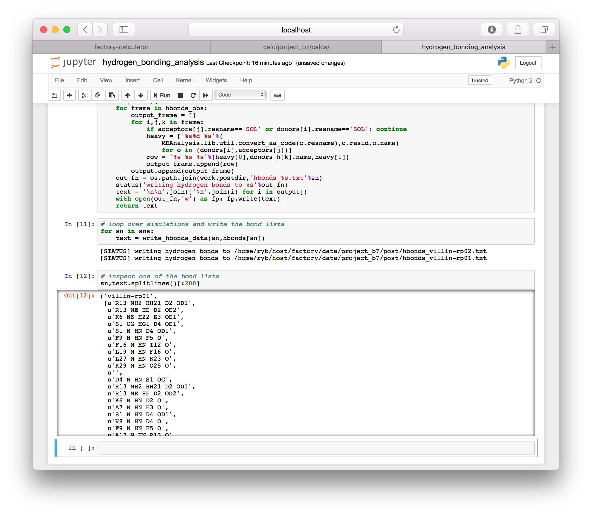
The hydrogen bonding script also contains a function which writes the hydrogen bonds to a text file in the post folder for your project (this is the same location where the slices are written, described in the instructions for downloading the trajectory). One text file is written for each simulation. The results for each frame are separated by blank lines. Each line contains the residue name and number for the donor and acceptor, with the name of the hydrogen in the middle. For example K6 NZ HZ2 E3 OE1 is the hydrogen bond from the NZ nitrogen and the HZ2 hydrogen on lysine K6 to the OE1 oxygen of glutamic acid E3 (we use one-letter amino acid codes).
4 Principal components analysis
This section tells you how to construct the file called
pca_analysis.ipynb, however we have already provided a copy of this notebook in your project calculation folder, so you only need to follow along and execute the script.
In this section we will perform the principal components analysis (PCA) for the motion of your protein. In contrast to previous sections, we will use a prepared set of data to perform the analysis in a Jupyter notebook. This is necessary because the PCA calculation requires a large sample consisting of many distinct frames of a trajectory, otherwise there will not be enough data to formulate a useful covariance matrix.
▶ Go to the calculator page and click the “interactive notebooks” link. Use the “new” button to make a new Python 2 notebook. Click the name of the notebook to change the name to something sensible, like pca_analysis.
4.1 Running commands in the termial
To compute the principal components, we will use a set of GROMACS tools which are typically accessed at the terminal. Jupyter allows you to call terminal (or “shell”, or more specifically BASH) commands directly from the notebook using an exclamation point. Very common commands (e.g. cd to change directory) do not require the exclamation point. Anytime you see an exclamation point in this section, it refers to a terminal command.
4.2 Getting the data
▶ We will begein by changing to our project’s data directory. Use the code in the following image to check your “present working directory” and then change to the equivalent data directory. Make sure that you select the right project folder. It will not be project_b7 as shown below, but it might be similar. You should also be careful to choose the right path. Some machines host your data with a different username than the one pictured below (ryb).
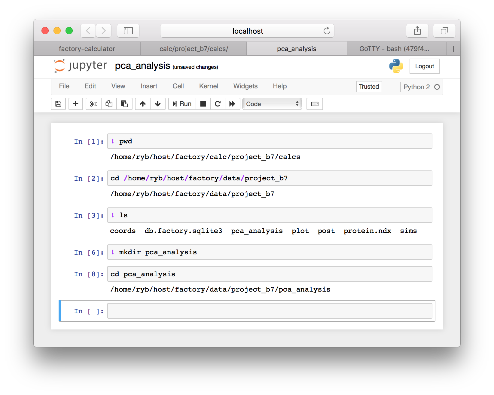
▶ Continuing to follow the image above, use ls to list the files in your project data folder and then make a new folder called pca_analysis using the mkdir command. Once you have completed the sequence above, you will have a folder to run our analysis. Change to the pca_analysis directory using the cd command after you make it.
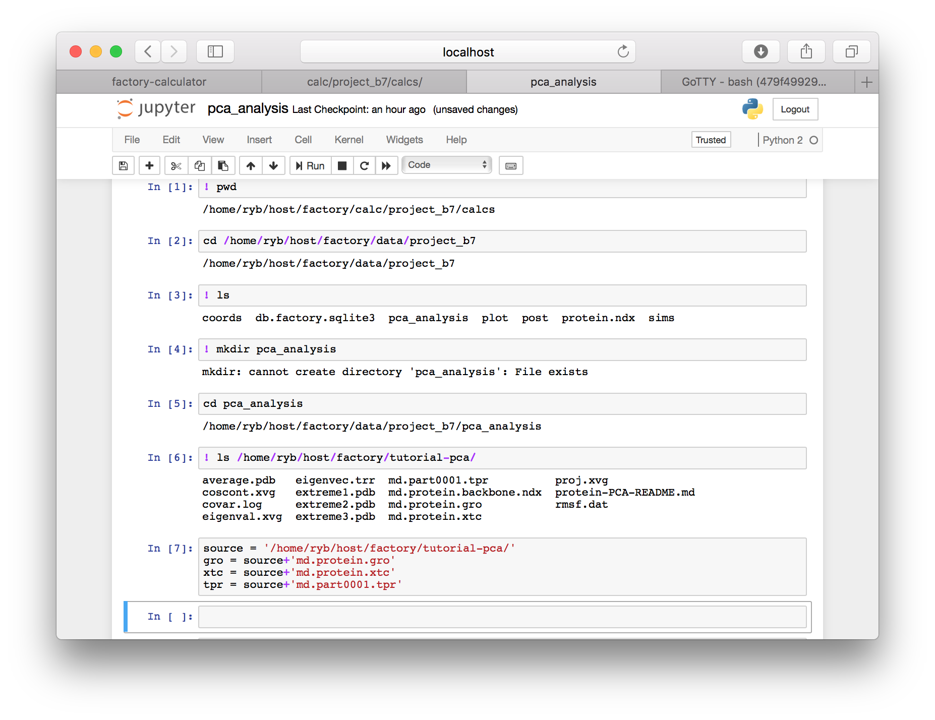
The factory resides inside a virtual machine on a remote server. We have placed a reference trajectory in factory/tutorial-pca. We will create python variables to point to the data.
▶ Add the following paths to a new cell. Note that the username (ryb) may be different on your server and the source variable must contain a trailing slash. These paths point to a shared dataset using the lysozyme protein which has run for a long time. Users who wish to analyze one of the simulations they have already created should skip this cell and see the instructions below.
# this cell points to a complete dataset for this demonstration
# to analyze a custom simulation, see the note in the PCA section
# ... titld "run PCA on a new simulation" for more details
source = '/home/ryb/host/factory/tutorial-pca/'
gro = source+'md.protein.gro'
xtc = source+'md.protein.xtc'
tpr = source+'md.part0001.tpr'
4.2.1 Run PCA on a new simulation
This sub-section is optional, and is meant for users who wish to analyze a new simulation instead of the shared data described above.
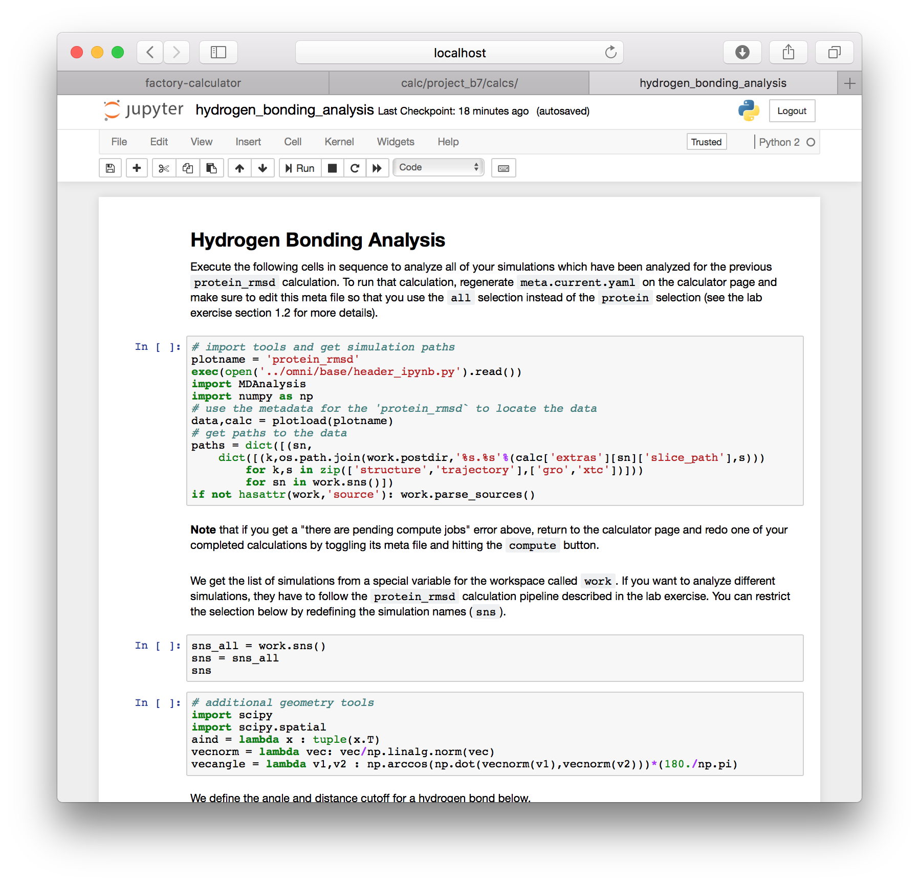
Instead of using the prepared dataset in the paths above, you may wish to use a simulation you already ran in the factory. To do this, add the following cell at the top of your notebook, before any cd commands, and replace the simulation name with your target.
# routine to import a custom simulation (select it below)
plotname = 'protein_rmsd'
exec(open('../omni/base/header_ipynb.py').read())
import MDAnalysis
import numpy as np
# use the metadata for 'protein_rmsd' to locate the data
data,calc = plotload(plotname)
# get paths to the data
paths = dict([(sn,
dict([(k,os.path.join(work.postdir,'%s.%s'%(calc['extras'][sn]['slice_path'],s)))
for k,s in zip(['structure','trajectory'],['gro','xtc'])]))
for sn in work.sns()])
# choose a simulation
sn = 'villin-rp01'
gro = paths[sn]['structure']
xtc = paths[sn]['trajectory']
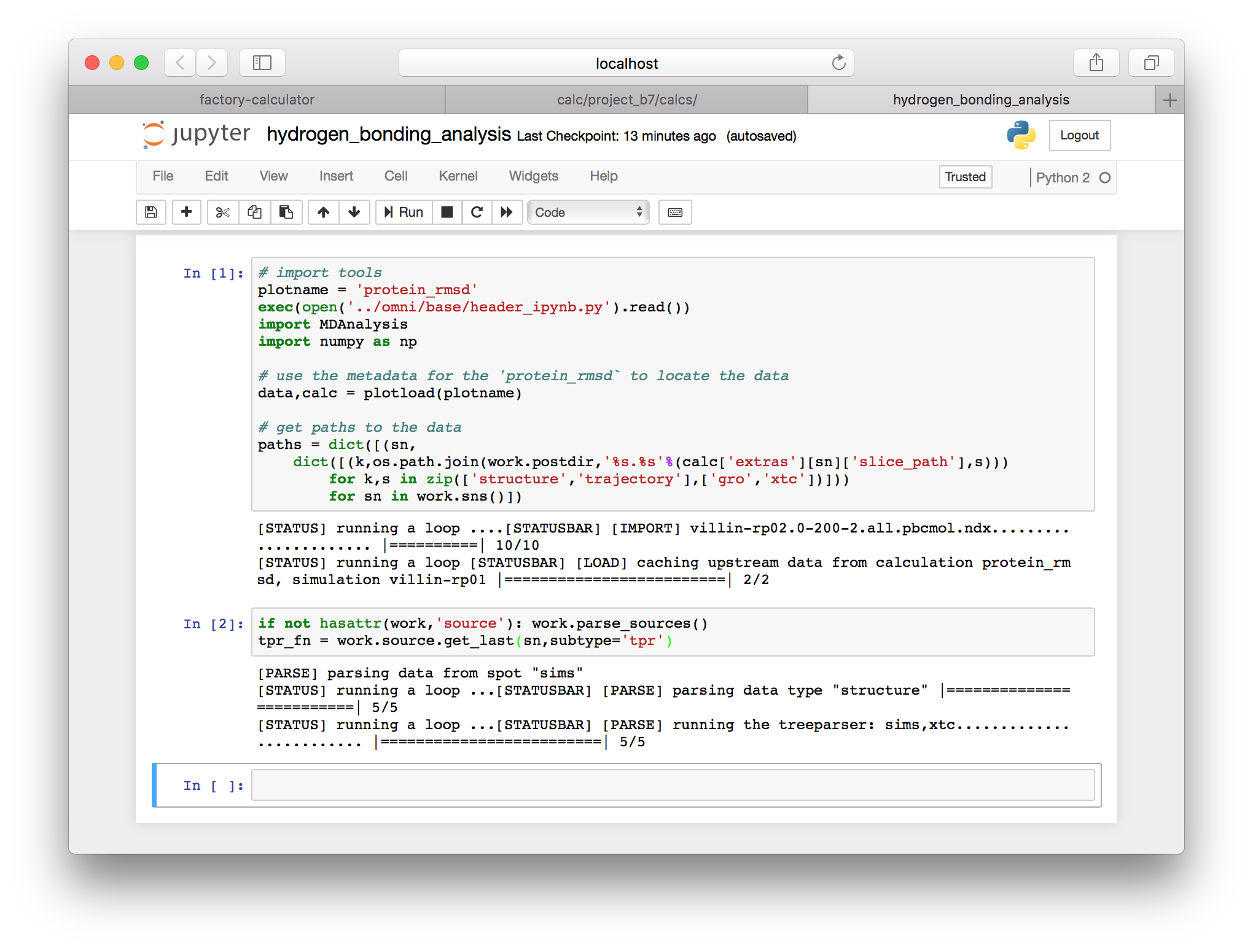
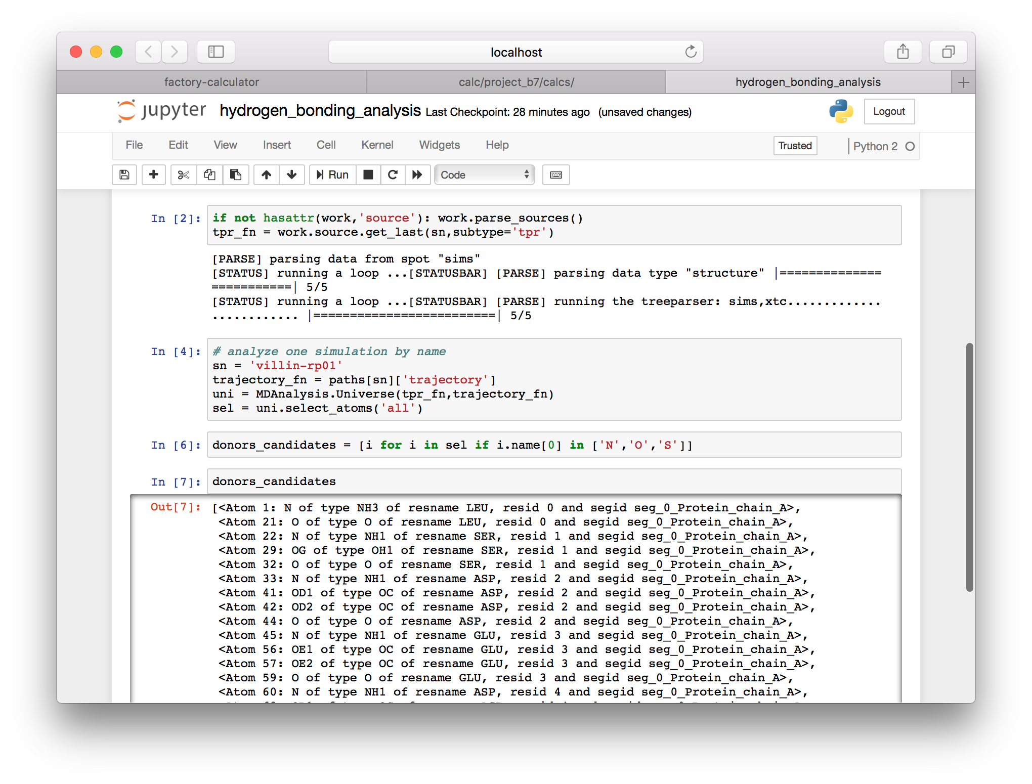
if not hasattr(work,'source'): work.parse_sources()
tpr = work.source.get_last(sn,subtype='tpr')To use a new simulation, you must generate the protein RMSD plot first, because this ensures that you have a valid trajectory to analyze. The appendix explains why. The example code below will retrieve data for the villin-rp01 simulation that I have already completed. As long as you do not redefine the gro, xtc, and tpr variables later in the script, then the remainder of the notebook will analyze your simulation, instead of the shared data.
4.3 Computing the principal components
Now we will study the principal components of the protein’s motion by calculating and diagonalizing the covariance matrix. First we will select a minimal subset of the protein backbone.
The Jupyter notebook allows you to access python variables in a bash command by enclosing them in braces. For example, the gro variable we defined above can be used in a terminal command via {gro}. You could also just as easily write the text of the variable into the command, but it is more convenient to use variables, particularly if you re-use the code with different data.
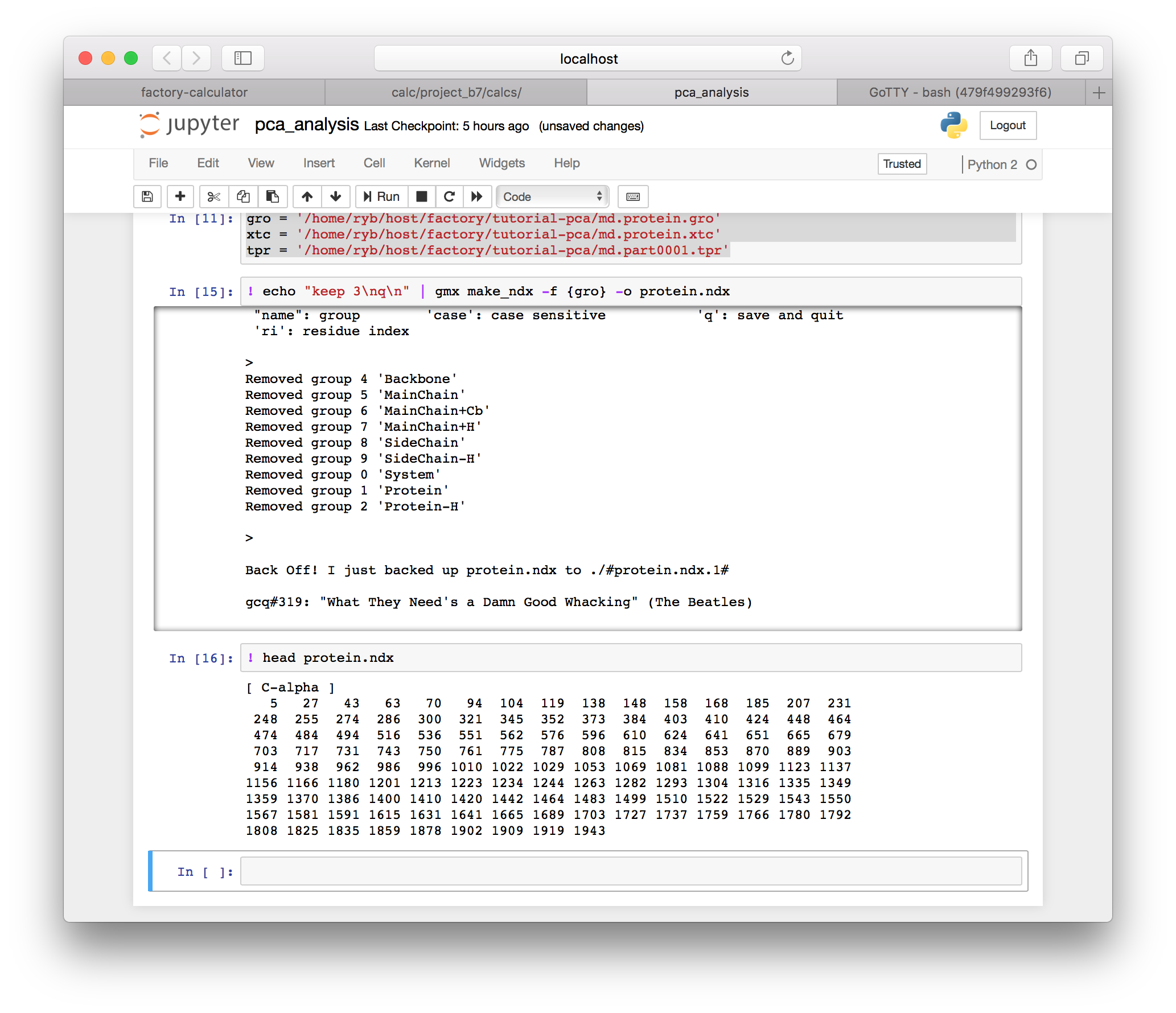
▶ Use the following GROMACS command (make_ndx) to select the protein. You can use the BASH head command to see the beginning of this file in the next cell.
! echo "keep 3\nq\n" | gmx make_ndx -f {gro} -o protein.ndxNote that the “pipe operator” (|) sends the preceding echo command to the gmx make_ndx program. This is equivalent to entering keep 3 followed by the return key, which is represented with a newline (\n) in the terminal. This takes the place of an interaction with the terminal program and allows us to run the code in the notebook.
▶ Next we will use the covar utility to generate the covariance matrix.
! gmx covar -f {xtc} -s {gro} -n protein.ndx
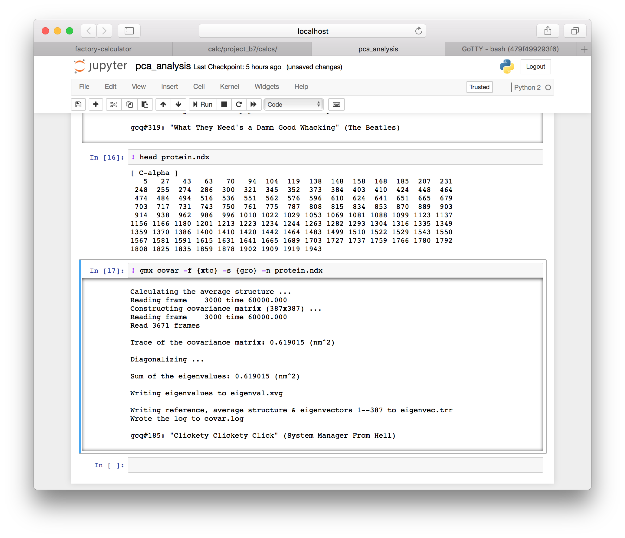
Our molecular dynamics simulation has produced a series of snapshots of the motion of an object with 3N-6 degrees of freedom. The covariance calculation effectively “compresses” this motion into a ranked list of orthogonal motions stored in eigenvec.trr. The eigenvectors with the largest eigenvalues correspond to the largest displacements, and the slowest fluctuations of the protein’s shape.
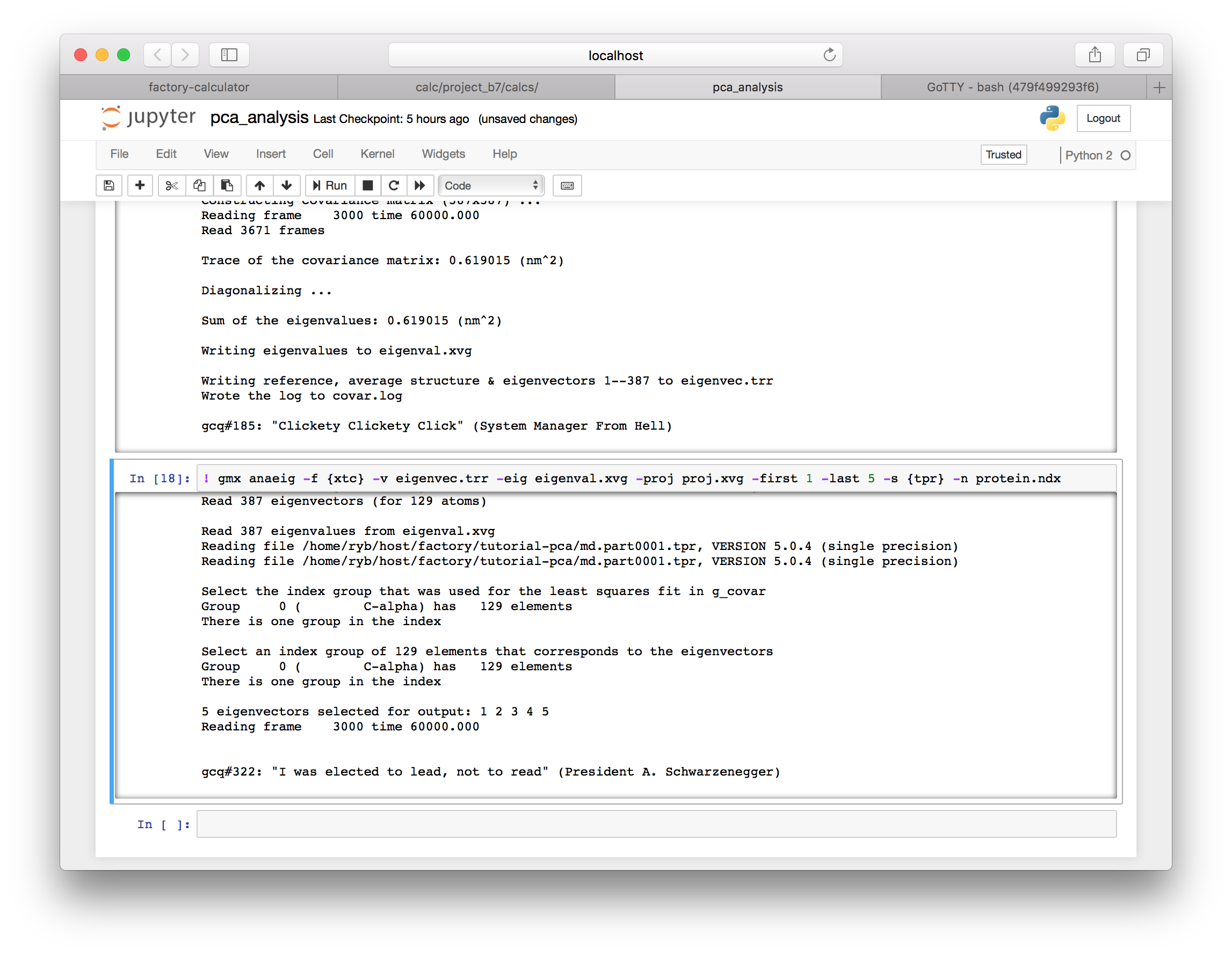
▶ Next we will use the anaeig utility to generate the first five principal components of the motion from the covariance matrix which was written to eigenvec.trr in the previous step. We will plot these in a moment.
! gmx anaeig -f {xtc} -v eigenvec.trr -eig eigenval.xvg -proj proj.xvg -first 1 -last 5 -s {tpr} -n protein.ndx
4.4 Plotting the spectrum
You can view the spectrum of eigenvalues by plotting eigenval.xvg. The eigenvectors with the largest eigenvalues capture explain the largest motions of the protein, while smaller eigenvalues capture less and less of the protein motion.
▶ Add the following cells to import plotting and analysis tools.
# import tools
%matplotlib inline
import matplotlib as mpl
import matplotlib.pyplot as plt
import numpy as np
▶ Use the following cell to read the eigenvalues written to eigenval.xvg in the previous section.
eigenvals = np.genfromtxt([i for i in open('eigenval.xvg').read().splitlines()
    if not i.startswith(('#','@'))])
▶ Use the following cell to plot the spectrum.
plt.plot(*eigenvals.T)
plt.xlabel('rank')
plt.ylabel('eigenvalue')
plt.yscale('log')
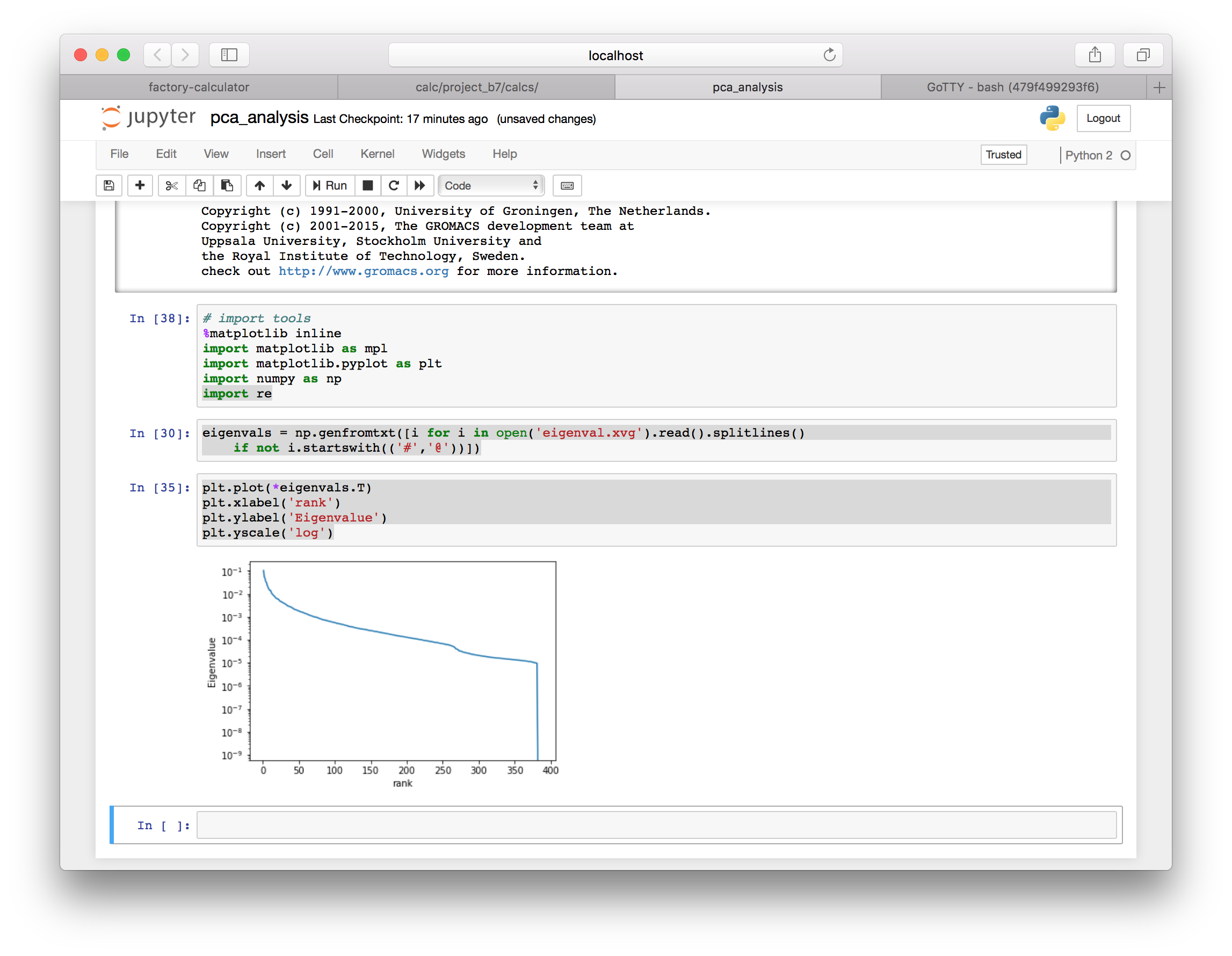
The spectrum tells us the magnitudes of the motion correspnding to each eigenvector. Next we will view the motion of the deviations along the top five eigenvectors.
4.5 Viewing the motion in VMD
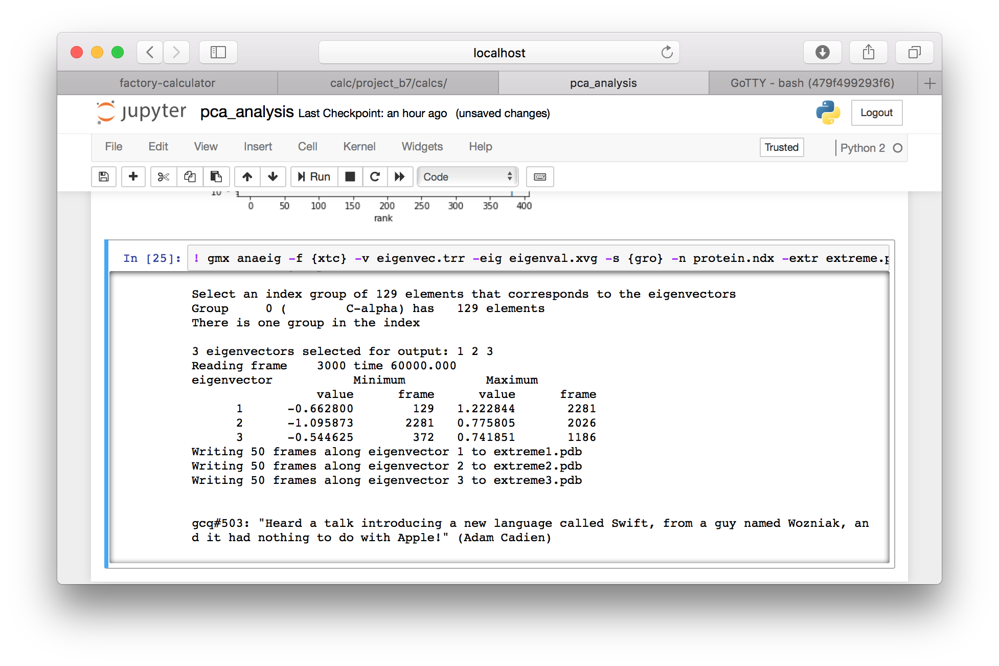
We can view the motion from each mode by using VMD. First, we will project the motion onto the average structure using the following command, which generates a 50-frame movie of the motion of each of the top three eigenvectors.
▶ Add a cell with the following GROMACS command.
! gmx anaeig -f {xtc} -v eigenvec.trr -eig eigenval.xvg -s {gro} -n protein.ndx -extr extreme.pdb -first 1 -last 3 -nframes 50
▶ Return to the calculator page, and use the “interactive notebooks” link to open the Jupyter server. Use the folder button (in the toolbar, to the left of your current path) to navigate to the root directory, and then navigate to the data directory, which should be located in subfolders data, your project folder e.g. project_XX, then data and pca_analysis.
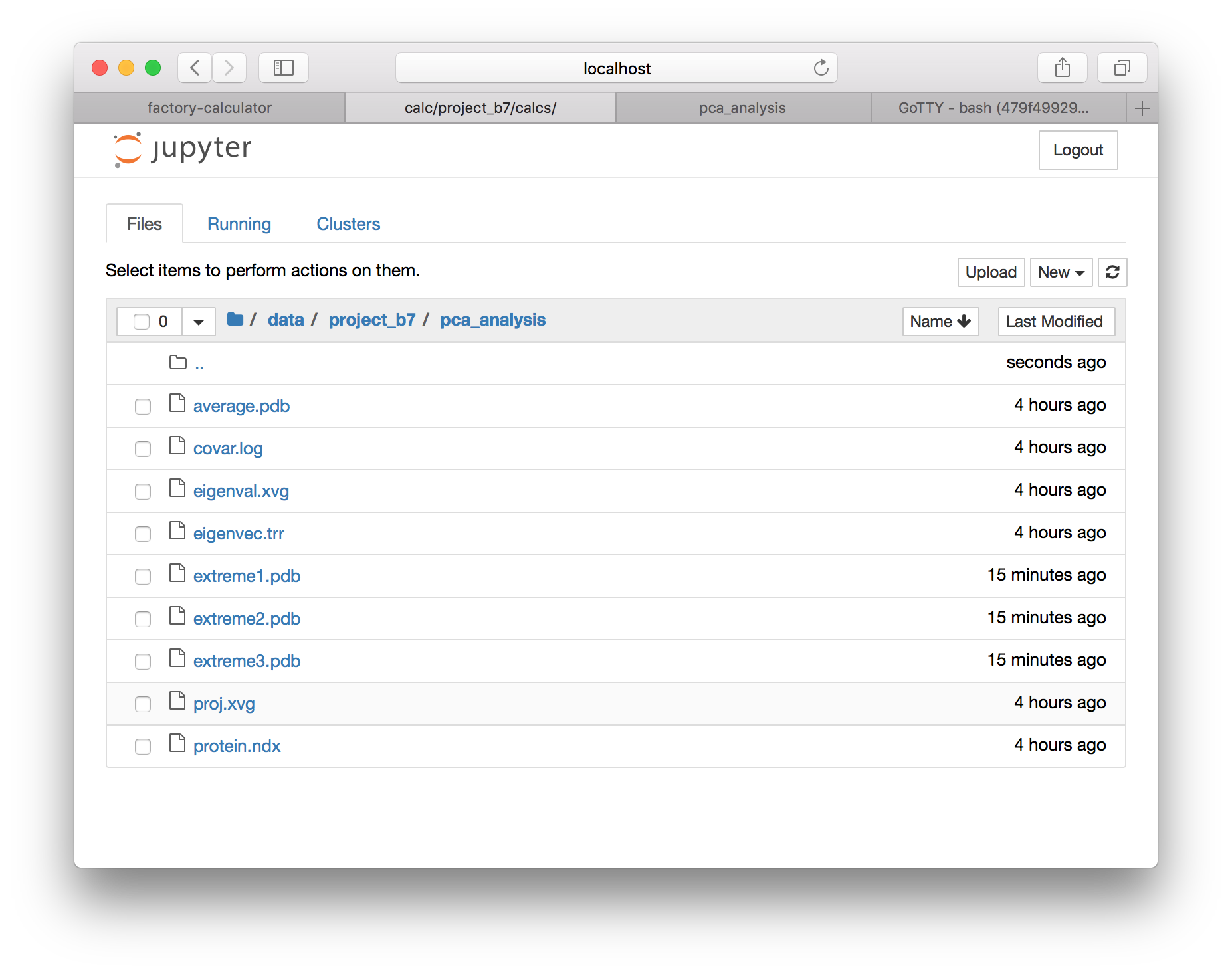
▶ Download extreme1.pdb (select the checkbox and use the download button) and open it in VMD. In the graphical representations window, change the drawing style to “points” and make them bigger. Then go to the trajectory tab, and draw multiple frames by entering 1:50, which will show all of the frames at once. Finally, go back to the “draw style” tab and color by the trajectory timestep. You can also inspect the other modes by downloading extreme2.pdb and extreme3.pdb.
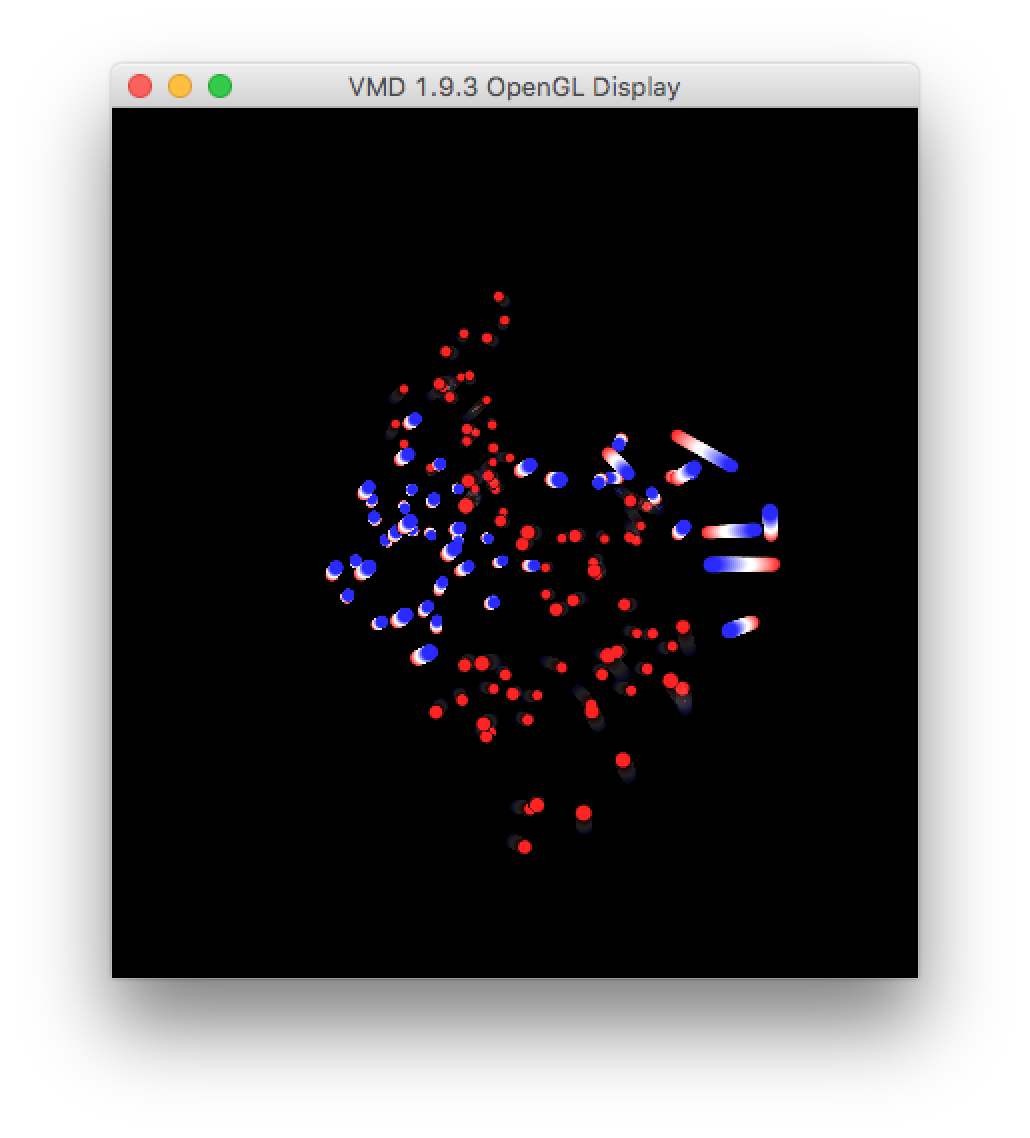
This visualization shows the motion of the largest eigenvector projected onto the average structure of the protein. The areas where the color changes the most, over the largest distance, emphasize the parts of the protein which fluctuate or “breathe” the most.
You can also visualize the motion by making a new representation (hide the old one by double-clicking it) and simply playing the video. It shows the large axis of the protein bending around the center “hinge” area.
4.6 Plotting the principal components
The principal components analysis approximates the motion of the protein as if it were evolving on an energy landscape shaped like a multidimensional harmonic well. If this model is valid, then the eigenvectors describe the various (orthogonal) fluctuations. In the previous section we visualized the motion of a single eigenvector. In our simulation, however, the protein’s motion is a superposition of many of these modes. Moreover, it does not necessarily follow a periodic oscillation in each of the modes, since the modes are inherently coupled to each other by the protein’s structure.
For this reason, we wish to inspect the motion of our simulation trajectory within or along each principal component. We can do this by first projecting the simulation trajectory onto the top five eigenvectors, and then measuring the time evolution of the displacement. We computed this earlier, in the command which generated proj.xvg. In this section we will plot it.
▶ Use the following code to parse the proj.xvg data we generated earlier. This code is somewhat complicated due to the formatting in this file.
with open('proj.xvg') as fp:
    text = '\n'.join([i for i in fp.read().splitlines()
        if not i.startswith(('#','@'))])
projections = [np.array([[float(m) for m in n.split()]
    for n in '\n'.join([i for i in z.split('\n') if i]).split('\n')])
    for z in text.split('\n&')]
▶ Use the following code to plot the motion along each of the top five eigenvectors.
fig,axes = plt.subplots(5,1,figsize=(10,10))
for pnum in range(5):
    ax = axes[pnum]
    ax.plot(*projections[pnum].T)
    ax.set_xlabel('frame')
    ax.set_ylabel('vector %d'%(pnum+1))
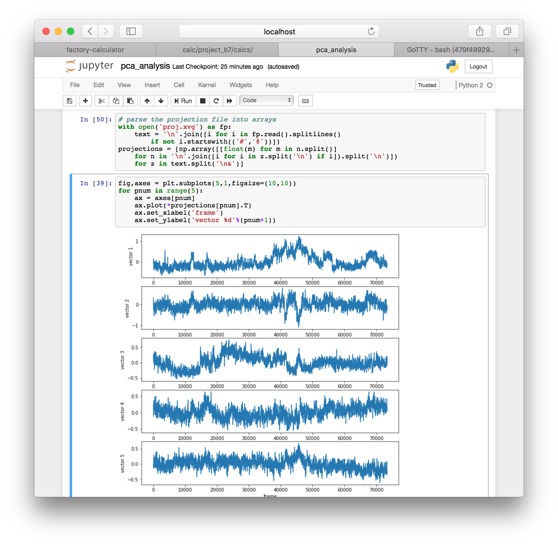
This command projects the motion of the protein along each of the top five eigenvectors and measures their deviations from the average structure in nanometers.
Appendix: custom calculations
The next two sections will show you how to construct new calculations inside the factory. The following examples will show you how to run calculations from earlier sections “by hand”, that is, without using code written by anybody else. We first demonstrate the code for a “manual” protein RMSD calculation which you completed earlier and then walk you through the hydrogen bonding analysis which formed the basis for the automatic code you used earlier to accomplish the same result. Users who are interested in writing other analyses not covered in this tutorial should follow these examples carefully and then use the general method to write their own code.
Note that anytime you want to run a custom calculation, you must compute the protein RMSD first because any new simulations must be processed with this code before we can get a copy of its trajectory.
Computing the RMSD “by hand”
At this point you have used the factory interface to create a slice or sample of a preexisting simulation, generated a plot of the RMSD, and downloaded the trajectory for further analysis. In this section, we will repeat the RMSD calculation “by hand” inside of a new notebook. This method can serve as an example for further calculations that you may wish to perform.
▶ From the calculator page, which may be open in a previous browser tab, click the interactive notebooks link in the upper left tile. On the notebook server page, click the New button and make a Python 2 notebook. Click the title of the notebook to rename it protein_rmsd_analysis.ipynb.
Now we will walk through the steps required to analyze the data. First we will import a few useful functions from the factory.
▶ Add the following code to a new cell and execute it.
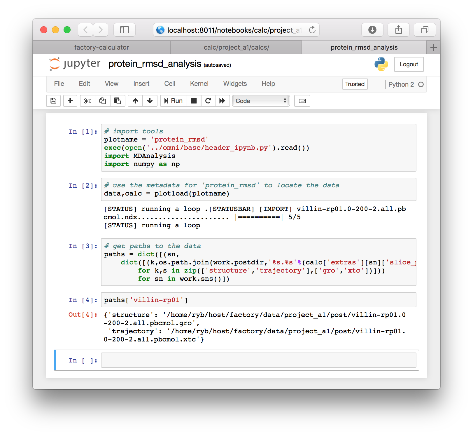
# import tools
plotname = 'protein_rmsd'
exec(open('../omni/base/header_ipynb.py').read())
import MDAnalysis
import numpy as np
▶ In another cell, use the plotload command to retrieve the protein RMSD data and the paths to our simulation trajectory.
# use the metadata for 'protein_rmsd' to locate the data
data,calc = plotload(plotname)
▶ Create a third cell using the following code to retrieve the paths to your data.
# get paths to the data
paths = dict([(sn,
    dict([(k,os.path.join(work.postdir,'%s.%s'%(calc['extras'][sn]['slice_path'],s)))
        for k,s in zip(['structure','trajectory'],['gro','xtc'])]))
        for sn in work.sns()])
The three cells above were specific to the factory, but they have provided us with the paths to our simulation “slices”. You can view these paths by typing paths['villin-rp01'] in a new cell which you can create with the “a” or “b” key to make the cell above or below the selected cell. The cell must be outlined blue instead of green for this to work. You can hit escape to change the cell outline to blue. Note that you should use your simulation name here, if it is different than the example.
At this point we have only retrieved the paths from the factory. In the next few cells we will read the trajectory using MDAnalysis, align the protein structure, and compute the RMSD directly.
We will start by creating an MDAnalysis Universe which points to the structure and trajectory files from our simulation.
▶ Add the following code to a new cell and execute.
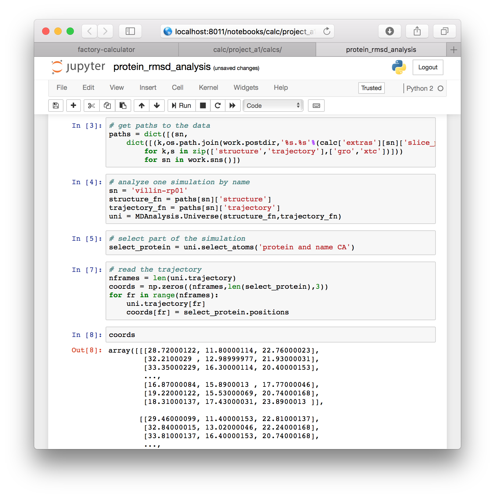
# analyze one simulation by name
sn = 'villin-rp01'
structure_fn = paths[sn]['structure']
trajectory_fn = paths[sn]['trajectory']
uni = MDAnalysis.Universe(structure_fn,trajectory_fn)
▶ In a new cell we will also create a selection object containing the coordinates of the protein alpha-Carbon atoms.
# select part of the simulation
select_protein = uni.select_atoms('protein and name CA')
▶ In the following cell, we will read the trajectory into a numpy array. Note that we have abbreviated the numpy library (which functions like MatLab) with the shorter name: np.
# read the trajectory
nframes = len(uni.trajectory)
coords = np.zeros((nframes,len(select_protein),3))
for fr in range(nframes):
    uni.trajectory[fr]
    coords[fr] = select_protein.positions
You can inspect the coordinates by typing coords into a new cell.
▶ Next we will use the following code to align the protein and compute the RMSD. The result is stored in a new variable called rmsds.
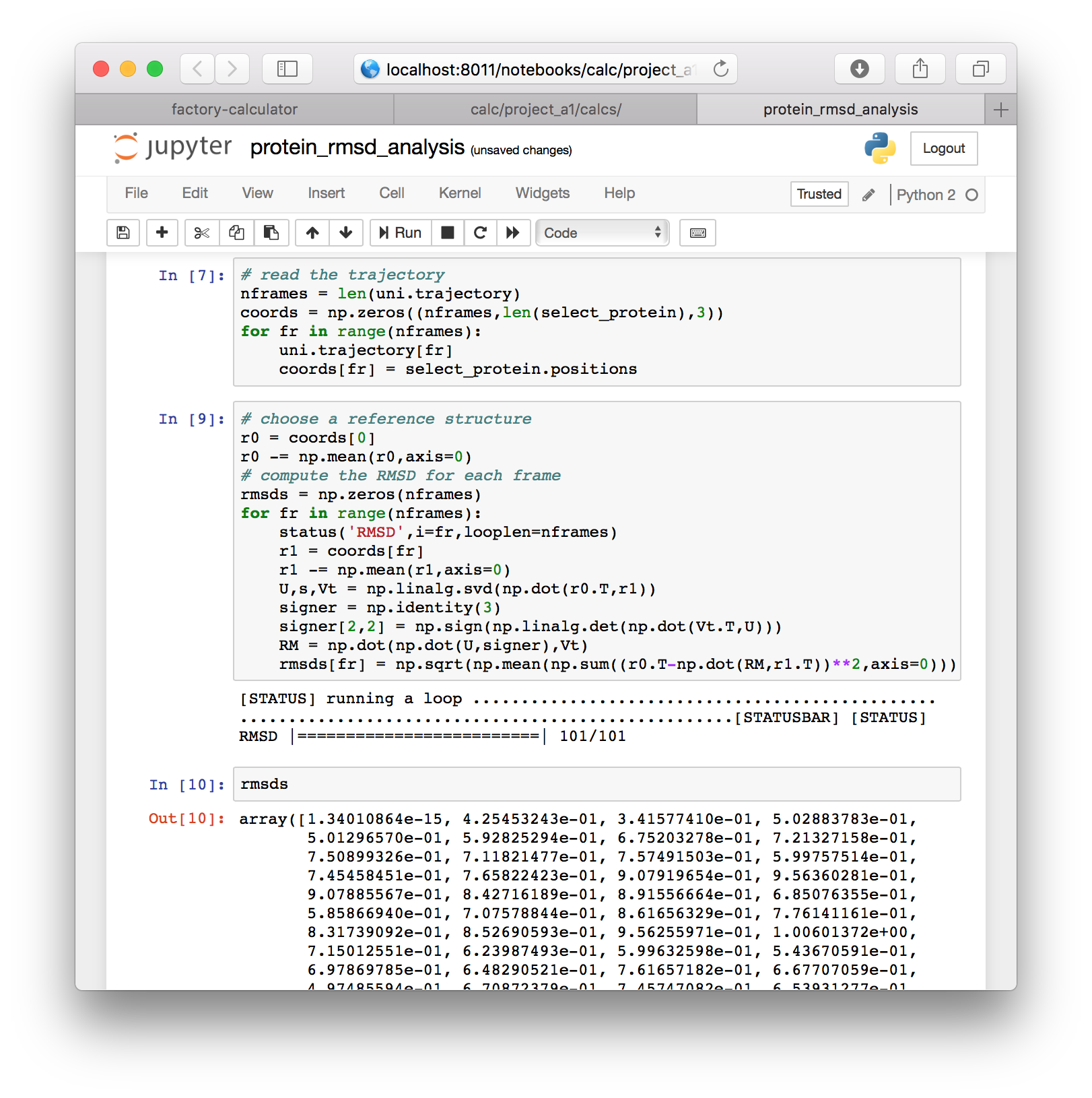
# choose a reference structure
r0 = coords[0]
r0 -= np.mean(r0,axis=0)
# compute the RMSD for each frame
rmsds = np.zeros(nframes)
for fr in range(nframes):
    status('RMSD',i=fr,looplen=nframes)
    r1 = coords[fr]
    r1 -= np.mean(r1,axis=0)
    U,s,Vt = np.linalg.svd(np.dot(r0.T,r1))
    signer = np.identity(3)
    signer[2,2] = np.sign(np.linalg.det(np.dot(Vt.T,U)))
    RM = np.dot(np.dot(U,signer),Vt)
    rmsds[fr] = np.sqrt(np.mean(np.sum((r0.T-np.dot(RM,r1.T))**2,axis=0)))
▶ Execute this cell and inspect the rmsds variable in a new cell.
▶ To view the data we will import the MatPlotLib software with the following code, in a new cell.
# import plot tools
%matplotlib inline
import matplotlib as mpl
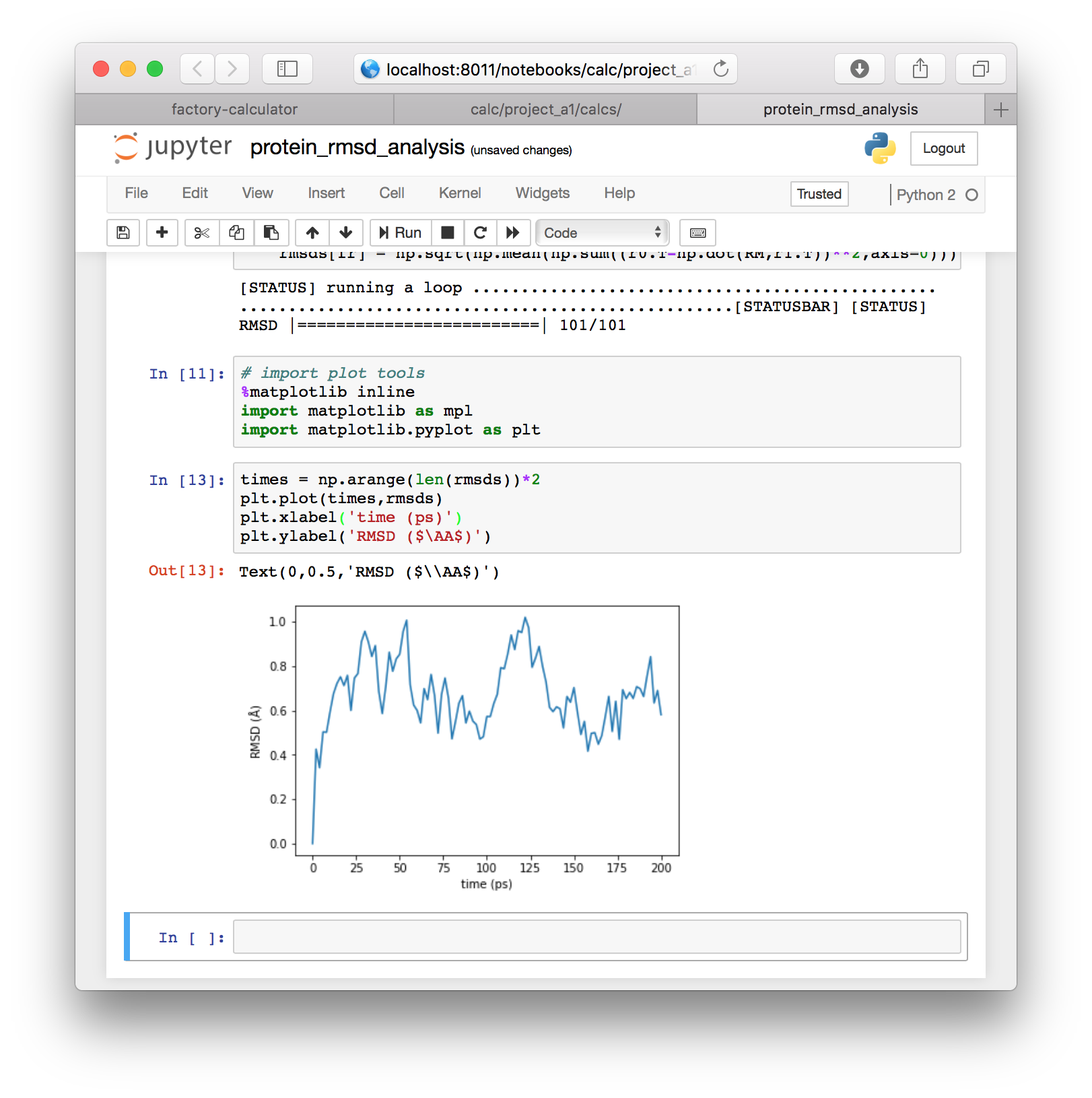
import matplotlib.pyplot as plt▶ Now that we have imported these tools, we can plot the data directly with the following code. We convert frames to times by multiplying by the 2ps sampling rate.
times = np.arange(len(rmsds))*2
plt.plot(times,rmsds)
plt.xlabel('time (ps)')
plt.ylabel('RMSD ($\AA$)')
The result will be plotted directly in the notebook. This plot will be identical to the one we generated automatically in the previous section.
In this section we used a few blocks of code to get the paths to our simulations from the factory. After that, we used only standard tools, namely MDAnalysis, numpy, and MatPlotLib to align our protein backbone positions and reproduce the RMSD calculation. This workflow serves as a basis for any other calculations you may wish to perform. Next, we will use a similar method to analyze the hydrogen bonds in our simulation.
Hydrogen bonding walkthrough
In the previous sections we learned how to execute and analyze simulations inside the factory. In the “download trajectory” section we also showed you how to download a sampled trajectory or “slice” that was generated in the course of computing the protein RMSD for your simulation. Users have three options for analyzing their data. Note that both options 2 and 3 require that you do option 1 first, because they use a sample of your trajectory called a “slice” which is written to disk.
- Run a “stock” calculation in the factory (e.g. protein RMSD which also generates a trajectory.
- Download the trajectory (from item 1) from a stock calculation and analyze it in another tool e.g. VMD.
- Use the trajectory (from item 1) to run a calculation “by hand” in a new Jupyter notebook (e.g. the “manual” protein RMSD calculation).
In this section we will compute the hydrogen bonds observed in your simulation using a method similar to item number 3 above. You must complete the protein RMSD calculation to continue.
Analyzing new simulations
Users frequently add more simulations. To analyze them, we need to add them to our metadata and generate new slices. In this subsection we will recap this procedure, however it is nearly identical to the method used above starting at with metadata preparation where we computed the protein RMSD.
▶ Return to the calculator page. Underneath the compute! button there should be a toggle for previous metadata such as meta.protein_rmsd.all.yaml. To make more metadata, we will press the “regenerate meta.current.yaml” button on the “meta files” tile. Note that this will overwrite the file, so it is always best to rename these files after you make them.
▶ Once you click the regenerate button, a new file with the familiar name meta.current.yaml will appear. Click the link to edit it and make sure that you click the title to rename it. You could use version numbers to indicate that this file is newer. In the example below I have renamed it meta.protein_rmsd.all.v2.yaml.
The image above shows that the factory has automatically detected all of the simulations I have run so far, including villin-rp01 and villin-rp02. Whenever new simulations are completed, you can regenerate metadata for them. Note that I have repeated the method we described in the metadata preparation section by changing all references to the protein selection to all so that the slices include all of the atoms and not just the protein.
▶ Save the modified file with ctrl+s or the File menu and close the tab to return to the calculator page. Note that you may need to click the text to “focus” it before saving, otherwise the browser may try to save the page as an HTML file instead.
▶ Select the toggle switch for your newly-created metadata, and click the compute! button to create slices for your new simulation and then run the protein RMSD calculation.
Whenver you want to add new simulations to your data, you should generate new metadata, toggle the file on the calculator page, and then run compute! with the large button. Do not select multiple meta files before computing. If you experience an error, you can always return to the calculator page (i.e. http://some.host:PORT/calculator/) and try again.
In this section we have updated our metadata to include new simulations, and generated new trajectories on disk as a byproduct of the protein RMSD calculation. You can download them using the method described in above.
Hydrogen bonding code
Users who made slices for all of their simulations in the previous section are welcome to download them (using the method above) and use other programs, like VMD, to measure the hydrogen bonds. In this section we will measure these bonds in a Jupyter notebook.
▶ Go to the calculator page and click the “interactive notebooks” link. On the notebook server page, make a new Python 2 notebook and rename it hydrogen_bonding_analysis.
▶ We will start with the same sequence as before. Add the following code to a new cell (or cells) at the top of your notebook.
# import tools
plotname = 'protein_rmsd'
exec(open('../omni/base/header_ipynb.py').read())
import MDAnalysis
import numpy as np

# use the metadata for the 'protein_rmsd` to locate the data
data,calc = plotload(plotname)

# get paths to the data
paths = dict([(sn,
    dict([(k,os.path.join(work.postdir,'%s.%s'%(calc['extras'][sn]['slice_path'],s)))
        for k,s in zip(['structure','trajectory'],['gro','xtc'])]))
        for sn in work.sns()])
▶ We will add two extra lines of code to retrieve the tpr file containing the connectivity of our bonds.
if not hasattr(work,'source'): work.parse_sources()
tpr_fn = work.source.get_last(sn,subtype='tpr')
Next we will choose a single simulation to analyze. For this example I will use sn = villin-rp01. Note that I will use sn to refer to the “simulation name” for the remainder of this exercise. In a previous cell we generated a dictionary called paths which contains the structure and trajectory paths on the server. The previous cell computed the tpr_fn, the filename for the run input TPR file.
▶ Use the following cell to use the trajectory file and the run input file to make an MDAnalysis Universe object and an associated atom selection.
# analyze one simulation by name
sn = 'villin-rp01'
trajectory_fn = paths[sn]['trajectory']
uni = MDAnalysis.Universe(tpr_fn,trajectory_fn)
sel = uni.select_atoms('all')
Note that MDAnalysis provides a very handy data structure. For example, we can loop through the sel object using a Python list comprehension (note that the list comprehension is extremely common in Python) and access the name attribute. In the next few cells we will use the various attributes of our selection (sel) to isolate the components in our system that can serve as hydrogen bond donors and acceptors.
▶ Use the following cell to identify hydrogen bond donors, which start with the letters N, O, or S. Note that the force field ensures that the atom names follow this convention.
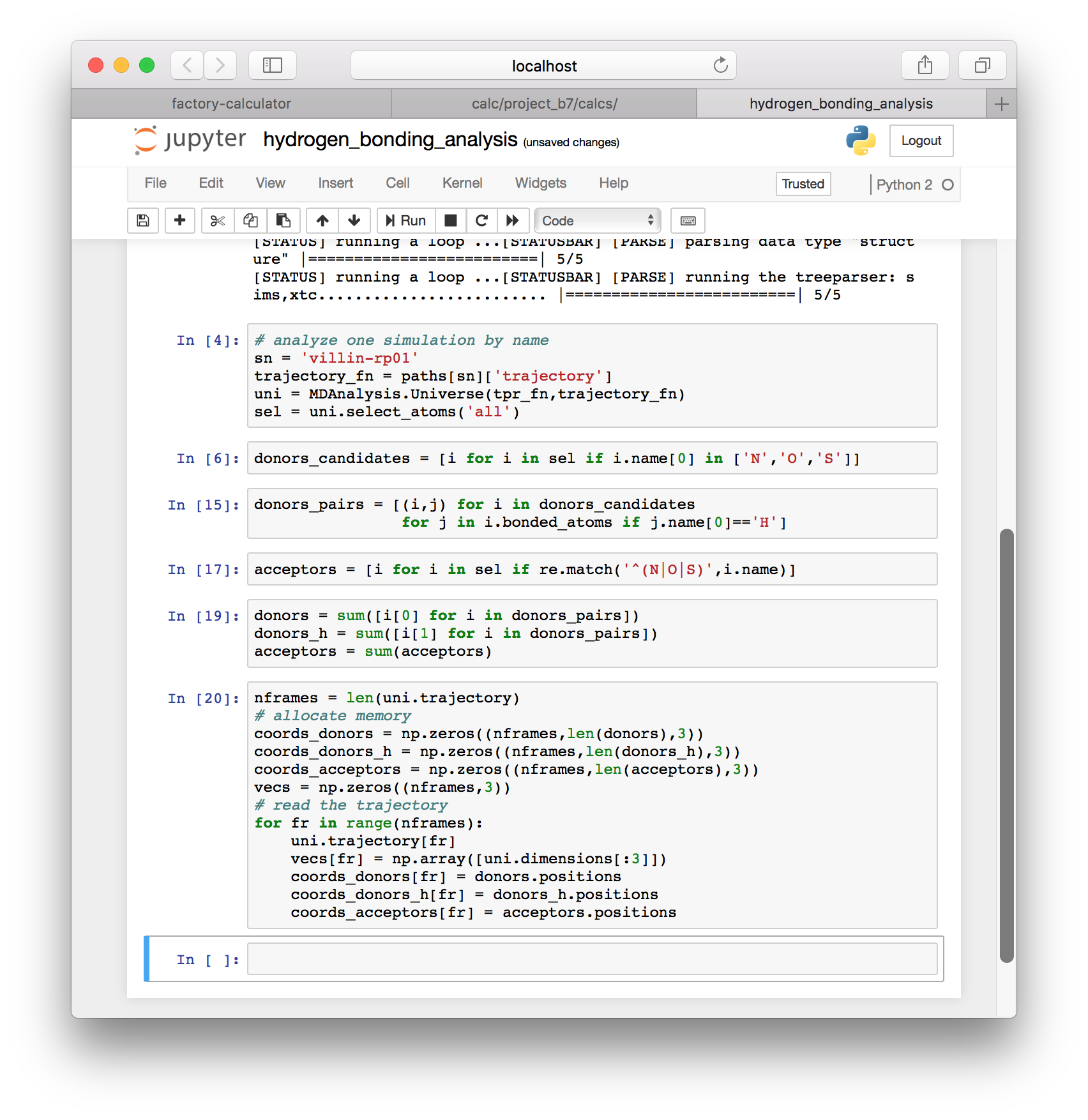
donors_candidates = [i for i in sel if i.name[0] in ['N','O','S'])]
▶ Use the bonded_atoms attribute in the following cell to identify hydrogen atoms that are bound to the donors.
donors_pairs = [(i,j) for i in donors_candidates
                for j in i.bonded_atoms if j.name[0]=='H']
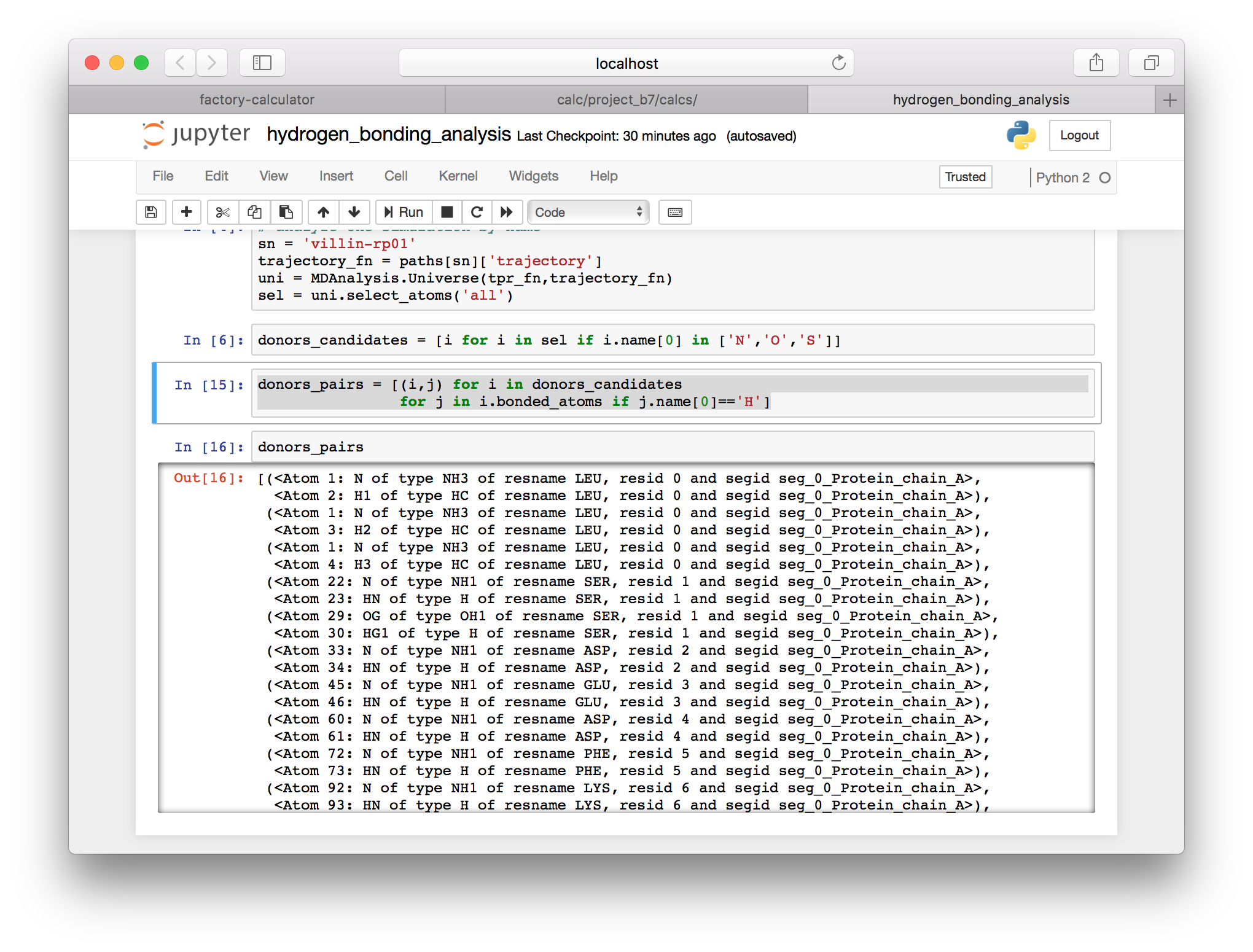
Note that Jupyter will display the last object in your cell (as long as you are not using the assignment operator = in that line). In the images above I have inspected some of the resulting items.
▶ Now that we have formulated a list of the possible donors, we can catalog the potential acceptors using the following cell.
acceptors = [i for i in sel if re.match('^(N|O|S)',i.name)]▶ To turn these selections into useful lists, we can use the sum command in Python. The MDAnalysis selections have special code which allows them to be “summed” or “concatenated” into larger selections.
donors = sum([i[0] for i in donors_pairs])
donors_h = sum([i[1] for i in donors_pairs])
acceptors = sum(acceptors)
▶ Use the following block of code to collect the coordinates for all of our donors and acceptors. Once we have the coordinates, we can use them to see which atoms are forming hydrogen bonds.
nframes = len(uni.trajectory)
# allocate memory
coords_donors = np.zeros((nframes,len(donors),3))
coords_donors_h = np.zeros((nframes,len(donors_h),3))
coords_acceptors = np.zeros((nframes,len(acceptors),3))
vecs = np.zeros((nframes,3))
# read the trajectory
for fr in range(nframes):
    uni.trajectory[fr]
    vecs[fr] = np.array([uni.dimensions[:3]])
    coords_donors[fr] = donors.positions
    coords_donors_h[fr] = donors_h.positions
    coords_acceptors[fr] = acceptors.positions
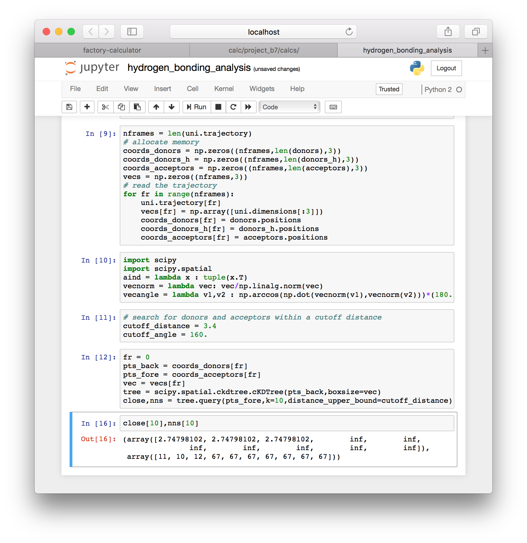
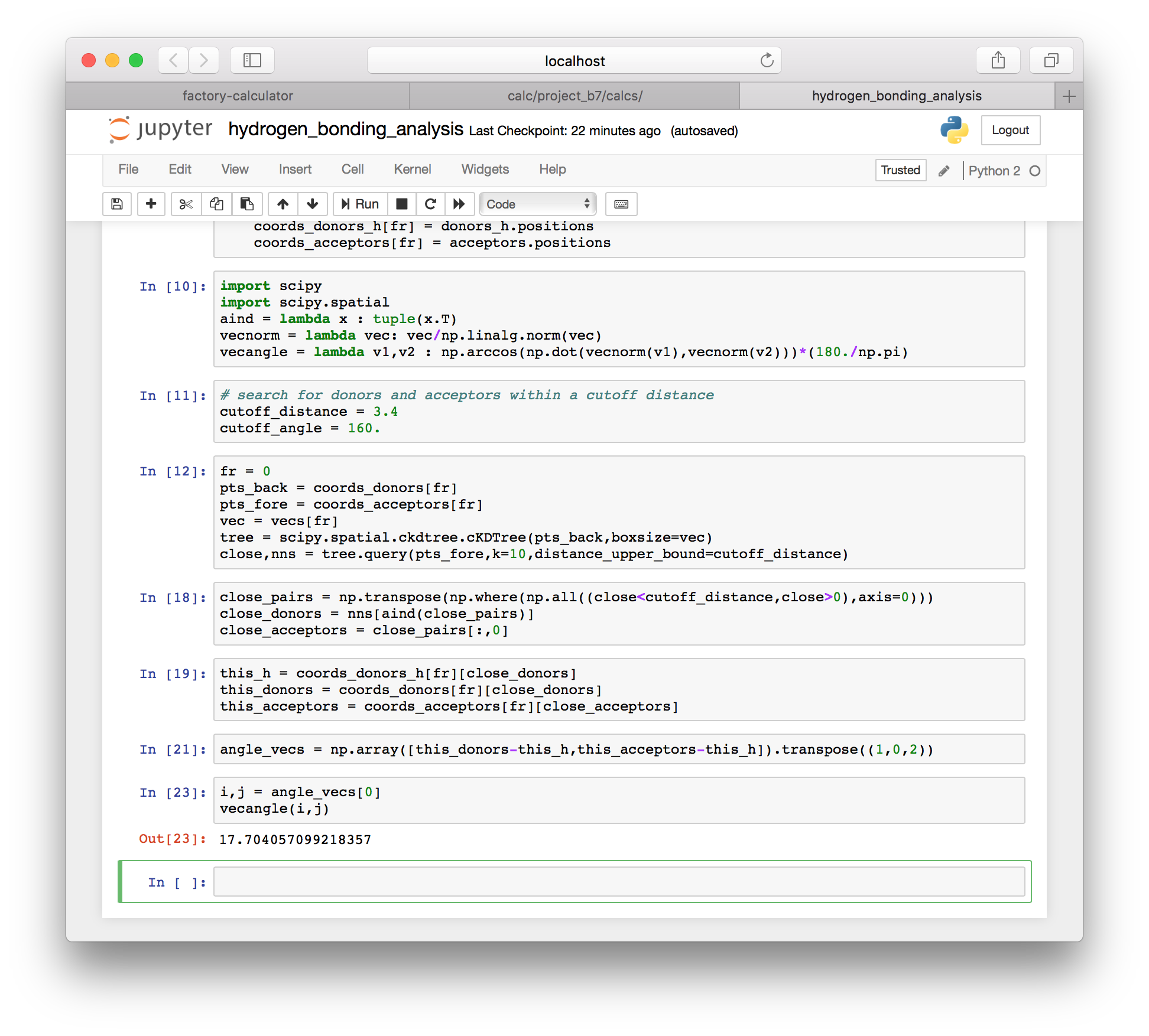
▶ Use the following cell to import the SciPy library (equivalent to MatLab) and define a few useful functions.
import scipy
import scipy.spatial
aind = lambda x : tuple(x.T)
vecnorm = lambda vec: vec/np.linalg.norm(vec)
vecangle = lambda v1,v2 : np.arccos(np.dot(vecnorm(v1),vecnorm(v2)))*(180./np.pi)
▶ Add the following cell to define a hydrogen bond, which must occur between heavy atoms within 3.4Å at an angle of 160° or more.
# search for donors and acceptors within a cutoff distance
cutoff_distance = 3.4
cutoff_angle = 160.
▶ In the next cell we will choose a frame (zero), select coordinates for the acceptors and donors, and construct a (periodic) K-D Tree to quickly measure the distances between the donors and acceptors.
fr = 0
pts_back = coords_donors[fr]
pts_fore = coords_acceptors[fr]
vec = vecs[fr]
tree = scipy.spatial.ckdtree.cKDTree(pts_back,boxsize=vec)
close,nns = tree.query(pts_fore,k=10,distance_upper_bound=cutoff_distance)
The code above constructs the tree and returns a list of the nearest neighbors (nns) and their distances. We search for the ten nearest acceptors to each donor (k=10). Use of the distance_upper_bound means that distances above the cutoff are reported as infinity.
▶ Use the following syntax to extract the donors that acceptors that are within the cutoff distance.
close_pairs = np.transpose(np.where(np.all((close<cutoff_distance,close>0),axis=0)))
close_donors = nns[aind(close_pairs)]
close_acceptors = close_pairs[:,0]
▶ Use the following syntax to extract the donors that acceptors that are within the cutoff distance.
this_h = coords_donors_h[fr][close_donors]
this_donors = coords_donors[fr][close_donors]
this_acceptors = coords_acceptors[fr][close_acceptors]
▶ The following cell will compute the vectors forming the angle between heavy atoms and the hydrogen.
angle_vecs = np.array([this_donors-this_h,this_acceptors-this_h]).transpose((1,0,2))▶ We can inspect this angle with the vecangle function.
i,j = angle_vecs[0]
vecangle(i,j)
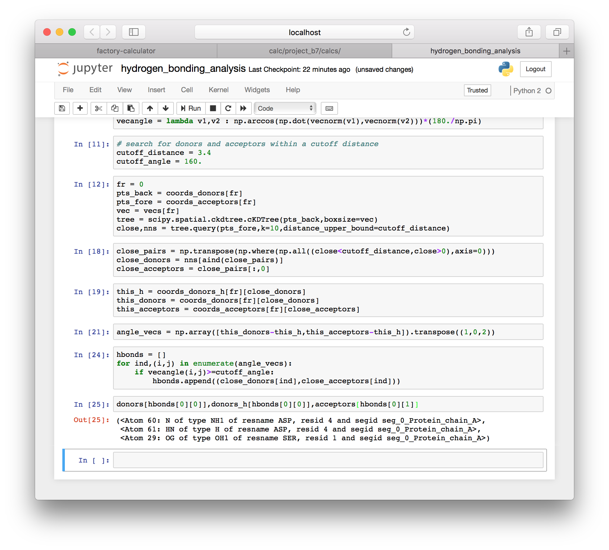
▶ We can sum up the hydrogen bonds by looping over all of the angle vectors between atoms that are within the distance cutoff and saving only those that have an angle larger than the angle cutoff. These are the valid hydrogen bonds.
hbonds = []
for ind,(i,j) in enumerate(angle_vecs):
    if vecangle(i,j)>=cutoff_angle:
        hbonds.append((close_donors[ind],close_acceptors[ind]))
▶ The method above computes a specific list of hydrogen bonds for a single frame, which we set in an earlier cell. We can inspect the first bond from the first frame using the following code.
donors[hbonds[0][0]],donors_h[hbonds[0][0]],acceptors[hbonds[0][1]]
While the specific bond list is important to us, we would also like to simply count the bonds in each frame of the simulation.
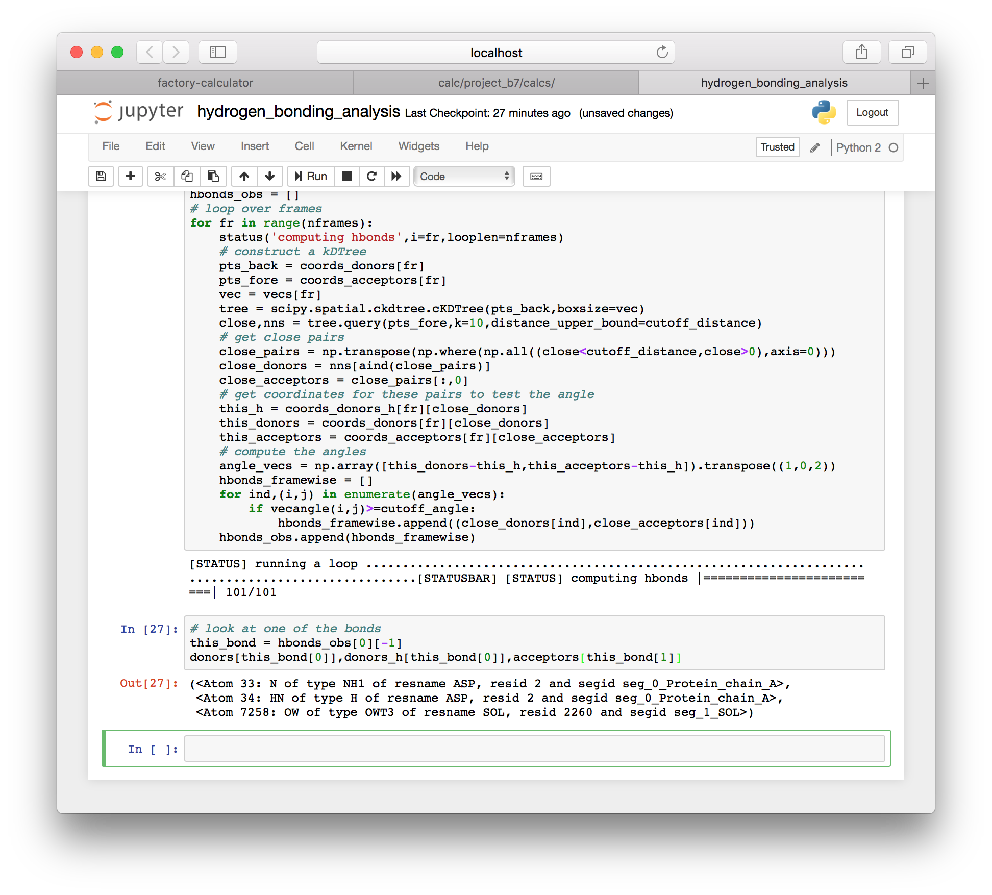
▶ Use the following cell, which combines the methods above, to count the hydrogen bonds.
# save each set of hbonds data to an item in a list
hbonds_obs = []
# loop over frames
for fr in range(nframes):
    status('computing hbonds',i=fr,looplen=nframes)
    # construct a kDTree
    pts_back = coords_donors[fr]
    pts_fore = coords_acceptors[fr]
    vec = vecs[fr]
    tree = scipy.spatial.ckdtree.cKDTree(pts_back,boxsize=vec)
    close,nns = tree.query(pts_fore,k=10,distance_upper_bound=cutoff_distance)
    # get close pairs
    close_pairs = np.transpose(np.where(np.all((close<cutoff_distance,close>0),axis=0)))
    close_donors = nns[aind(close_pairs)]
    close_acceptors = close_pairs[:,0]
    # get coordinates for these pairs to test the angle
    this_h = coords_donors_h[fr][close_donors]
    this_donors = coords_donors[fr][close_donors]
    this_acceptors = coords_acceptors[fr][close_acceptors]
    # compute the angles
    angle_vecs = np.array([this_donors-this_h,this_acceptors-this_h]).transpose((1,0,2))
    hbonds_framewise = []
    for ind,(i,j) in enumerate(angle_vecs):
        if vecangle(i,j)>=cutoff_angle:
            hbonds_framewise.append((close_donors[ind],close_acceptors[ind]))
    hbonds_obs.append(hbonds_framewise)
As with the method for a single frame, this method produces a list of hydrogen bond donors. However, it appears to include some solvent, as you can see when we inspect the last bond (-1) in the first frame (0).
# look at one of the bonds
this_bond = hbonds_obs[0][-1]
donors[this_bond[0]],donors_h[this_bond[0]],acceptors[this_bond[1]]
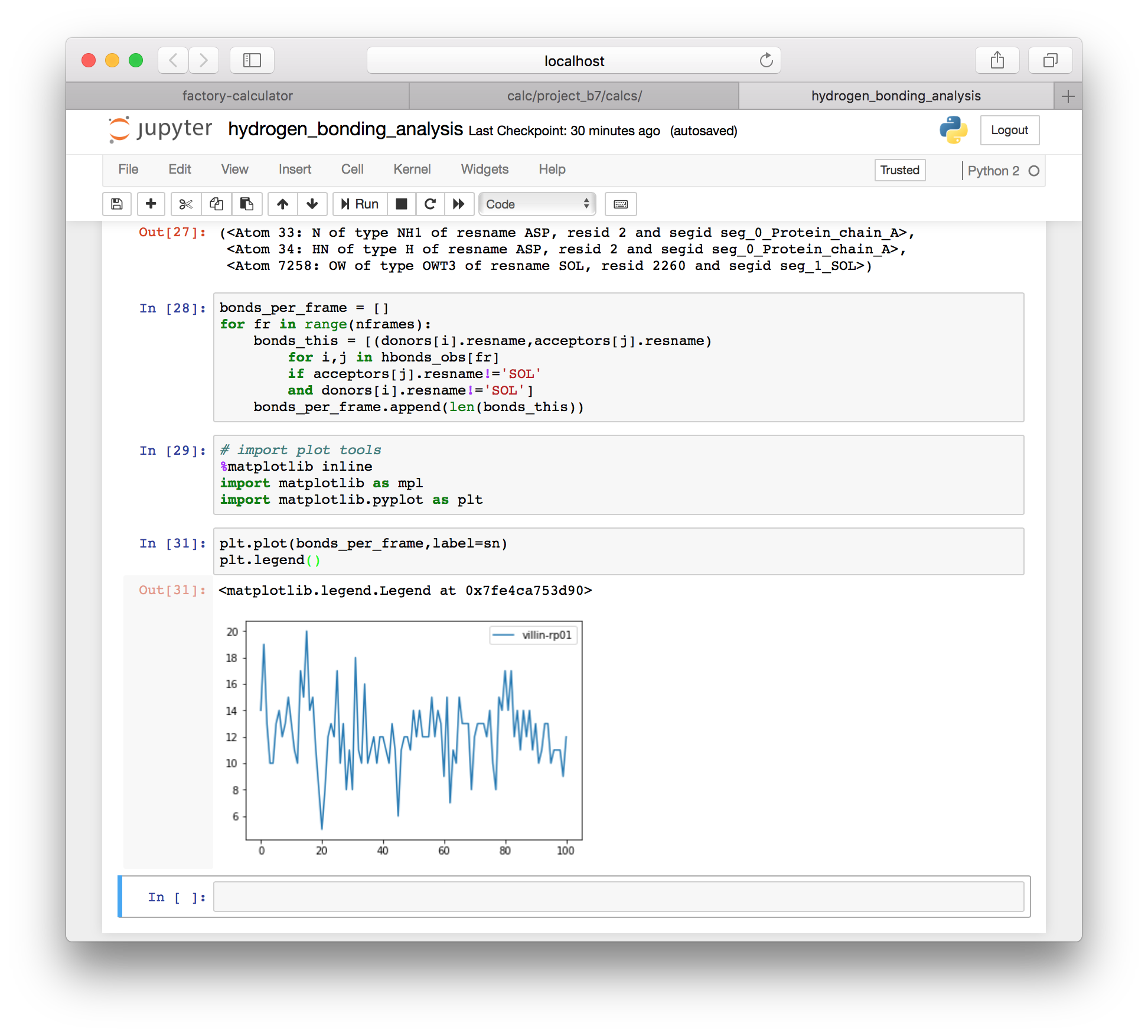
▶ Filter out bonds involving solvent using the following code.
bonds_per_frame = []
for fr in range(nframes):
    bonds_this = [(donors[i].resname,acceptors[j].resname)
        for i,j in hbonds_obs[fr]
        if acceptors[j].resname!='SOL'
        and donors[i].resname!='SOL']
    bonds_per_frame.append(len(bonds_this))
▶ Import the plot libraries with the following code.
# import plot tools
%matplotlib inline
import matplotlib as mpl
import matplotlib.pyplot as plt
▶ Since we computed a count of the hydrogen bonds in each frame (minus those with solvent) we can use the MatPlotLib plotter to visualize the total number of bonds over time.
plt.plot(bonds_per_frame,label=sn)
plt.legend()
Now that we have an observed bond list (hbonds_obs) we can isolate and view any hydrogen bonds in the system. You are also free to use other simulation names in the analysis above to compare one simulation to another.