This feature allows users to run simulations from inside of an [IPython/Jupyter] notebook.

The factory consists of a framework for managing calculation projects with a graphical layer that lets users do this quickly and systematically. You can use the factory in a text-only mode to manage calculations for preexisting datasets but you can also use the graphical interface to make the simulations and directly analyze them in a single pipeline.

Besides offering a fairly rapid, self-contained method for running AUTOMACS simulations and directly analyzing them, the pipeline also has a fairly basic queue system, which means that you can prepare several simulations which will execute in sequence. The authors have found that this method works best on a workstation where you prepare jobs, start equilibration, and them move them to a supercomputer.

Since the queue runs inside the graphical interface, however, it is less obvious how the underlying code works. This means that users should already be familiar with AUTOMACS to understand how the factory starts a simulation.

To ensure that users know how the system works, we also offer a “manual” method inside the graphical interface, which prepares an AUTOMACS simulation and lets you run it inside a notebook. This scheme gives you the best of both worlds: you can run a simulation in the pipeline, but you can also see exactly how it is executed.

The factory interface is a fairly superficial wrapper around automacs and omnicalc, not least of all because its authors (Ryan and Joe) are not professional interface designers. This means that running the code in the notebook is almost identical to running it from the terminal. In both cases, AUTOMACS does the fairly menial work, including copying files, keeping logs of what has already happened, and importing modular functions. Whether you use the interface to start a simulation, your terminal, or the notebook, the result is still the same.

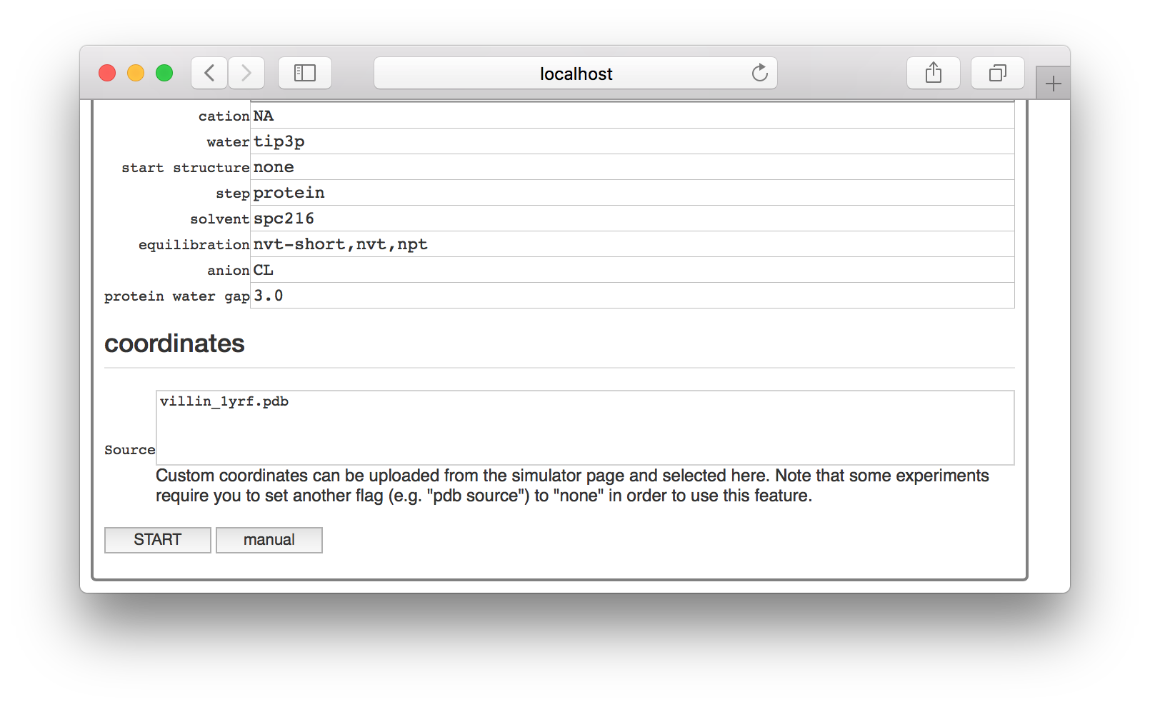
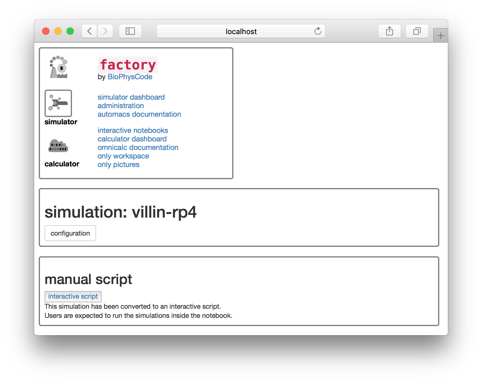
To run a simulation in a notebook, start with the method described in the single pipeline but you should stop before clicking “start” on the settings page of your simulation. You will notice a “manual” button next to it.

This button will generate a new simulation notebook and provide you with a button to open it. Note that we serve the factory interface on one port, and the notebook on another. The “interactive script” button will take you to the notebook server.

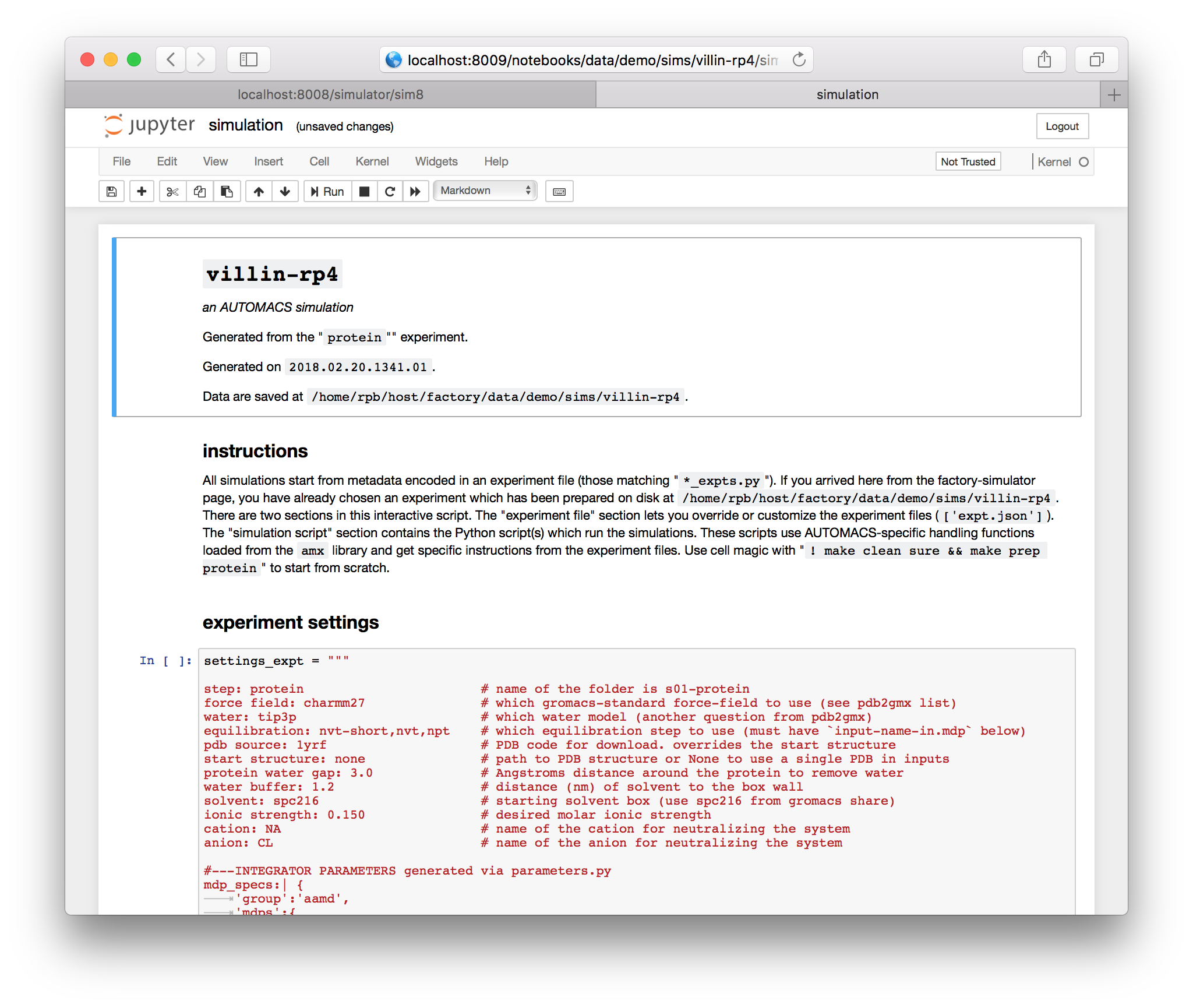
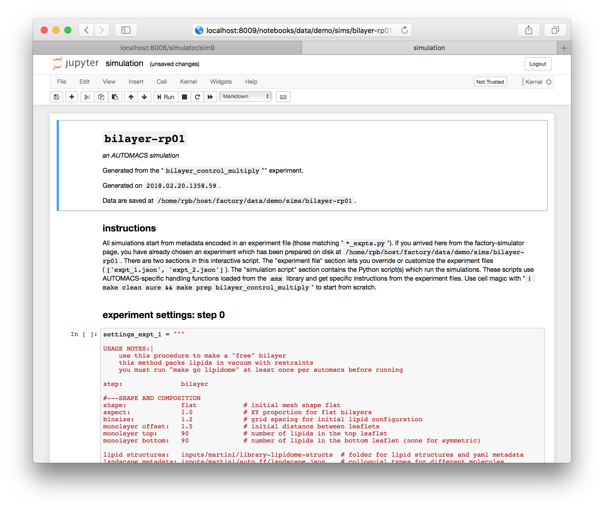
When you selected an experiment earlier, automacs ran the make prep <experiment_name> command on disk. This prepared the expt.json and script.py files on disk, which are the two ingredients necessary to run an automacs simulation. You could run python script.py from the terminal to run the simulation with the default settings.

The notebook gives you a chance to edit the settings before you run the script. The settings are typically stored as dictionary literals in files with the suffix _expts.py e.g. protein_expts.py. While each experiment has a few important settings, including the location of the script it uses, the settings block contains the parameters important to the simulation. You can edit them in a cell which overwrites the expt.json file.

When you are ready, you can run the script, which has been copied into a cell. You are free to leave the browser while it runs. If you return, you will notice an hourglass in the browser tab. Note that the hourglass is present on firefox, but might not be visible on other browsers, in which case you should just leave the browser open until it is complete.

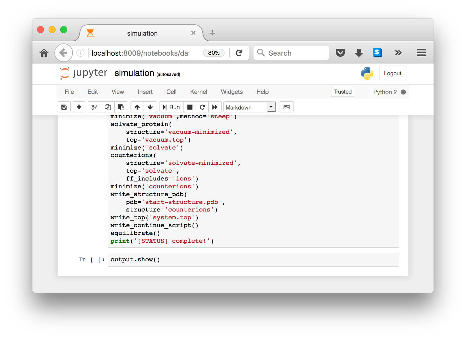
To ensure that the notebook can run after you leave the browser, we capture output in a variable so that you can take a look at it when you return. The final cell shows the output via output.show().

Some automacs simulations include multiple steps. We call these “metaruns”, and they are given a separate category when you select your experiment. The notebook executes each step in sequence. The only real difference is that you end up with multiple scripts and settings files e.g. script_1.py and expt_1.json.

Using the simulation notebooks described in this section is nearly identical to using the old-fashioned text and terminal method. Users who like the notebooks are encouraged to try the standalone terminal method too.