Simulation-analysis pipeline

This walkthrough covers the use of the factory as a single pipeline for creating and analying simulations. To run the walkthrough, users must first create a factory and then create a new omnicalc project. There is both a quickstart guide and [unit test]/validation/#create_factory) available for starting the factory. All paths in this guide are relative to the factory location. Next we will explain how to set up a new omnicalc project, and after that, we will run a simulation and analyze it inside the graphical user interface.

Making a new omnicalc project

This section outlines the method for creating a factory project and serving it locally. It mimics a [unit test]/validation/#demo_serve) which can be used to serve a factory over the web from inside a Docker. Note that this guide is similar to the quickstart guide for calculations, except we will use the graphical user interface (GUI) to generate simulation data directly. In both cases, we must start by making a new omnicalc project.

An omnicalc project is described by a “connection” file which tells omnicalc where to store simulations, how to serve an instance of the factory, and where to store post-processing data and plots. Once you have [created a factory]/validation#create_factory), make a directory called factory/connections and prepare a connection file called connect_demo.yaml with the following contents.

# FACTORY PROJECT (the base case example "demo")
demo:
# include this project when reconnecting everything
enable: true 
site: site/PROJECT_NAME  
calc: calc/PROJECT_NAME
calc_meta_filters: ['specs_demo_meta.yaml','meta.current.yaml']
repo: http://github.com/biophyscode/omni-basic
database: data/PROJECT_NAME/db.factory.sqlite3
post_spot: data/PROJECT_NAME/post
plot_spot: data/PROJECT_NAME/plot
simulation_spot: data/PROJECT_NAME/sims
port: 8000
port_notebook: 8001
public:
  port: 8008
  notebook_port: 8009
  # use "notebook_hostname" if you have a router or zeroes if using docker
  notebook_hostname: '0.0.0.0'
  # you must replace the IP address below with yours
  hostname: ['555.555.55.55','127.0.0.1']
  credentials: {'detailed':'balance'}
# import previous data or point omnicalc to new simulations, each of which is called a "spot"
# note that prepared slices from other integrators e.g. NAMD are imported via post with no naming rules
spots:
  # colloquial name for the default "spot" for new simulations given as simulation_spot above
  sims:
    # name downstream postprocessing data according to the spot name (above) and simulation folder (top)
    # the default namer uses only the name (you must generate unique names if importing from many spots)
    namer: "lambda name,spot=None: name"
    # parent location of the spot_directory (may be changed if you mount the data elsewhere)
    route_to_data: data/PROJECT_NAME
    # path of the parent directory for the simulation data
    spot_directory: sims
    # rules for parsing the data in the spot directories
    regexes:
      # each simulation folder in the spot directory must match the top regex
      top: '(.+)'
      # each simulation folder must have trajectories in subfolders that match the step regex (can be null)
      # note: you must enforce directory structure here with not-slash
      step: '([stuv])([0-9]+)-([^\/]+)'
      # each part regex is parsed by omnicalc
      part: 
        xtc: 'md\.part([0-9]{4})\.xtc'
        trr: 'md\.part([0-9]{4})\.trr'
        edr: 'md\.part([0-9]{4})\.edr'
        tpr: 'md\.part([0-9]{4})\.tpr'
        # specify a naming convention for structures to complement the trajectories
        structure: '(system|system-input|structure)\.(gro|pdb)'

The project name is given at the top of the connection file: demo and will replace any instance of PROJECT_NAME in the text. The paths above are relative to ./factory/ but you can use absolute paths to store the plots (plot_spot) and post-processing data (post_spot) elsewhere. These paths can be changed later if you move your data, by rerunning the connect command below.

The sims dictionary tells omnicalc where to find simulation data. It is currently set to the default value for using a single simulation-analysis pipeline, however you can also use this dictionary to import preexisting simulation data by following the calculation guide. Each entry e.g. sims tells omnicalc where to look for data, while the regular expressions (“regexes”) tell it how to interpret files on disk as trajectory files, structure files, etc.

Above the spots dictionary are entries for port and notebook_port. These are set to the default location for serving a local copy of the factory to e.g. http://localhost:8000. If this port is not available, choose one that is. If you wish to serve the factory over the internet, you will need to use root access to open the required ports, update the public dictionary with the right ports, and then add your IP address to the hostname list. We recommend doing this with a [unit test inside of docker]/validation#demo_serve) for security reasons.

Once you have prepared the connection file, run the following commands to start the factory.

make connect demo
make run demo

The make run command will provide you with a web address for the running factory. Later you can stop the factory with make shutdown demo. If you wish to serve the factory over the web, run the following commands. The web address should be obvious from your hostname and the ports you selected in the connection file.

make connect demo public
make run demo public

You can reconnect as many times as you want since this procedure does not erase any data. You can reconnect to change the factory to a public port, or to change paths. You can run as many factory projects as you want and then stop them individually with make shutdown demo or together with make shutdown. Since these jobs run in the background, you can also use make show_running_factories to see their process ID numbers.

In the following walkthrough we will be using codes which have been shared on github at the omni-basic repository. These files were shared according to instructions in the calculation guide. We told omnicalc to clone this repository by setting the repo key in the connection file. If you instead set repo: calc/PROJECT_NAME/calcs then omnicalc will make a blank repository at factory/calc/demo/calcs for you to add your calculations instead. This guide uses preexisting codes as a demonstration.

The method above corresponds to the [demo serve unit test]/validation#demo_serve), while the remainder of the guide is meant to be performed on the web interface.

Running a simulation

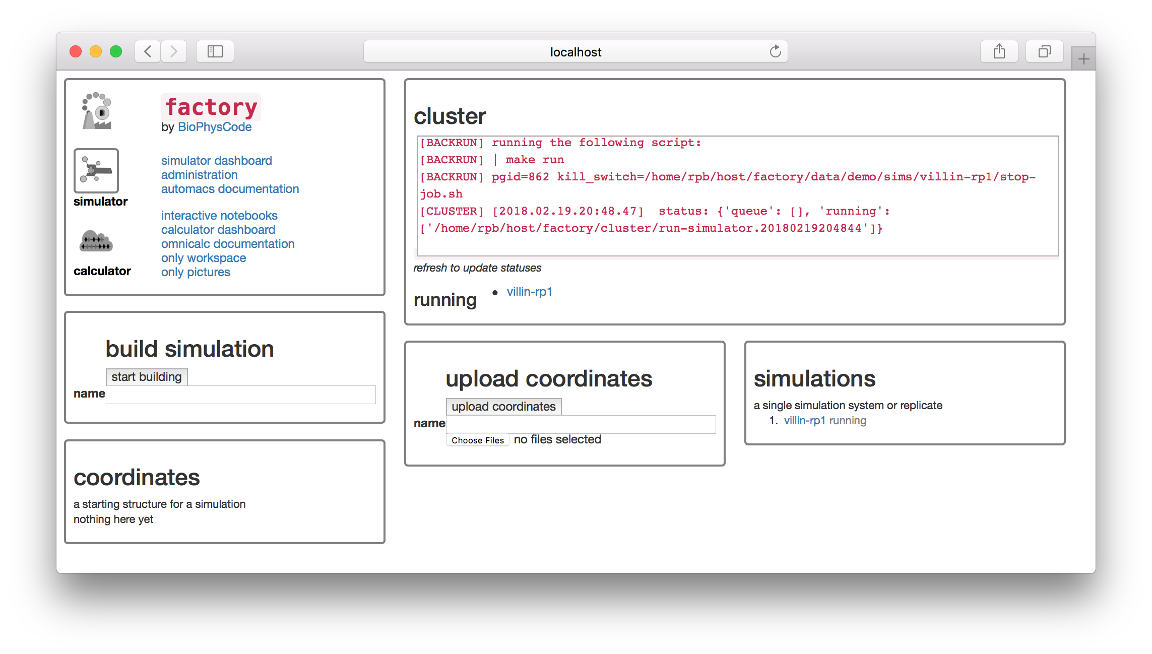
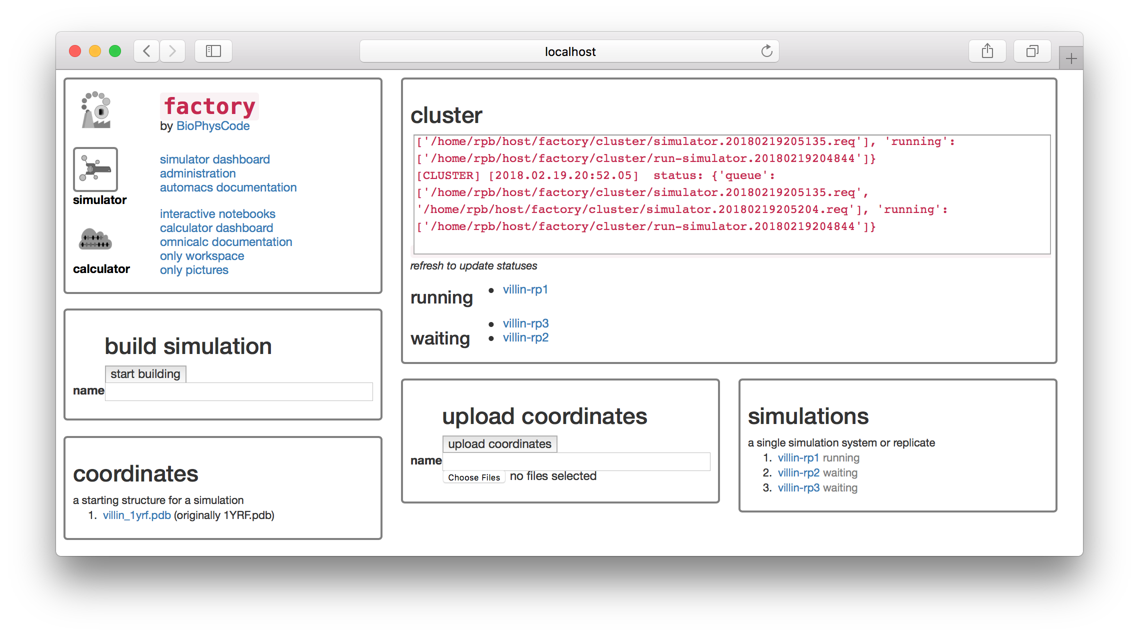
In this section, we will run and analyze a protein simulation. Once you have served the factory, open it in a browser. If you are running it locally on port 8000 then visit http://localhost:8000 otherwise select the same port you used above. You should see the following screen.

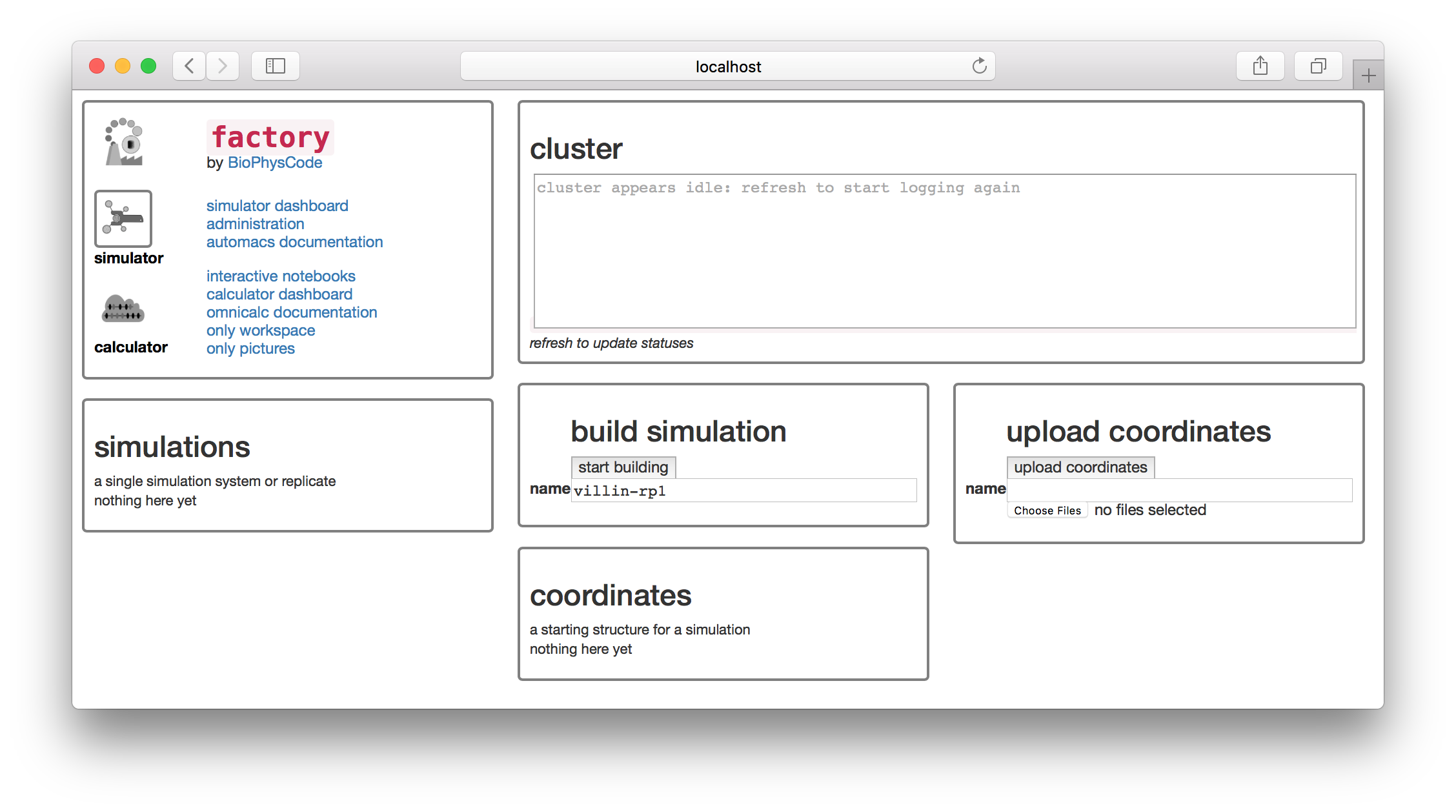
Let’s build a simulation of the villin headpiece. Name the first replicate villin-rp1 as shown above. Never use spaces in a name, since these names are used for folders on disk. Click the build simulation button to continue. The next page offers a set of “kickstarters” which correspond to select extra code modules which can be loaded into automacs.

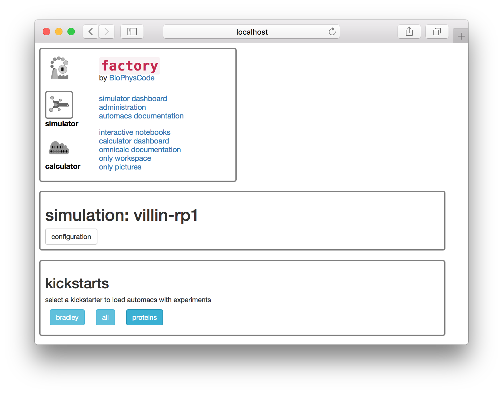
Select the proteins kickstarter on the page shown below. The next page offers a list of experiments. These experiments come along with the automacs modules.

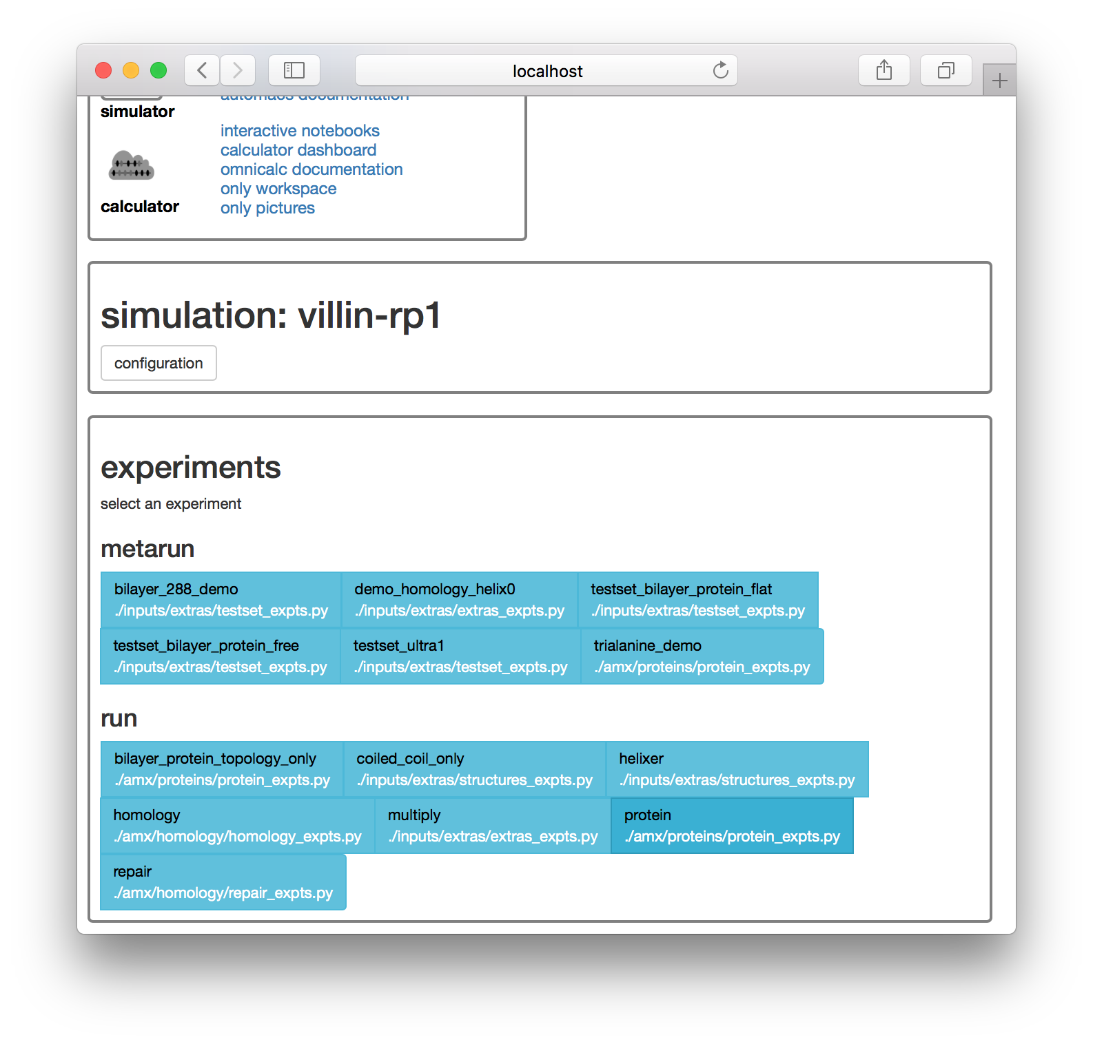
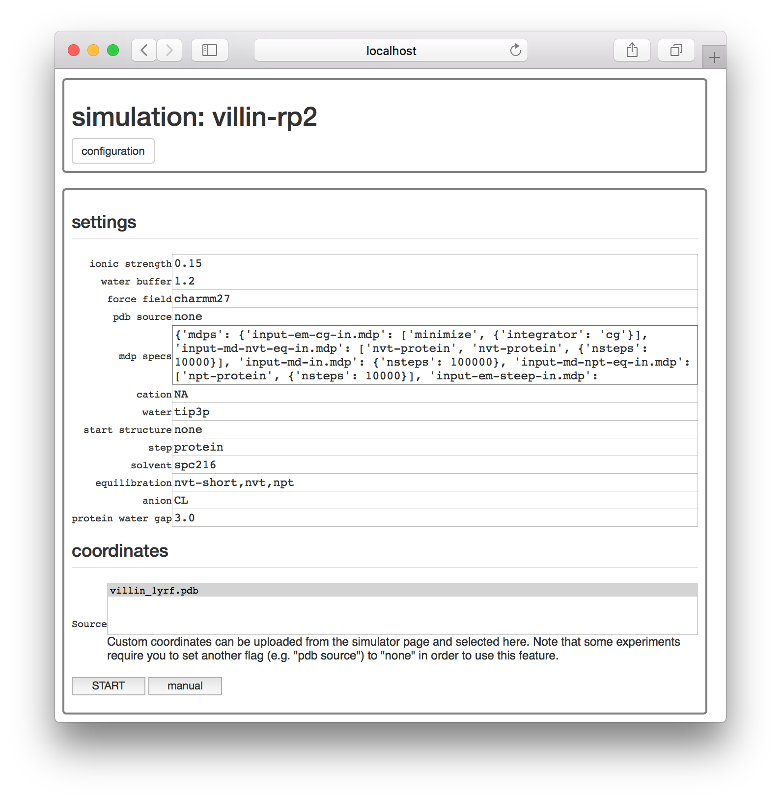
Click the protein experiment in the “run” list shown above. The next page provides a number of options for setting up the simulation including the ionic strength of the solvent, the distance between the protein and the periodic boundary (called the “watter buffer”, in nanometers).

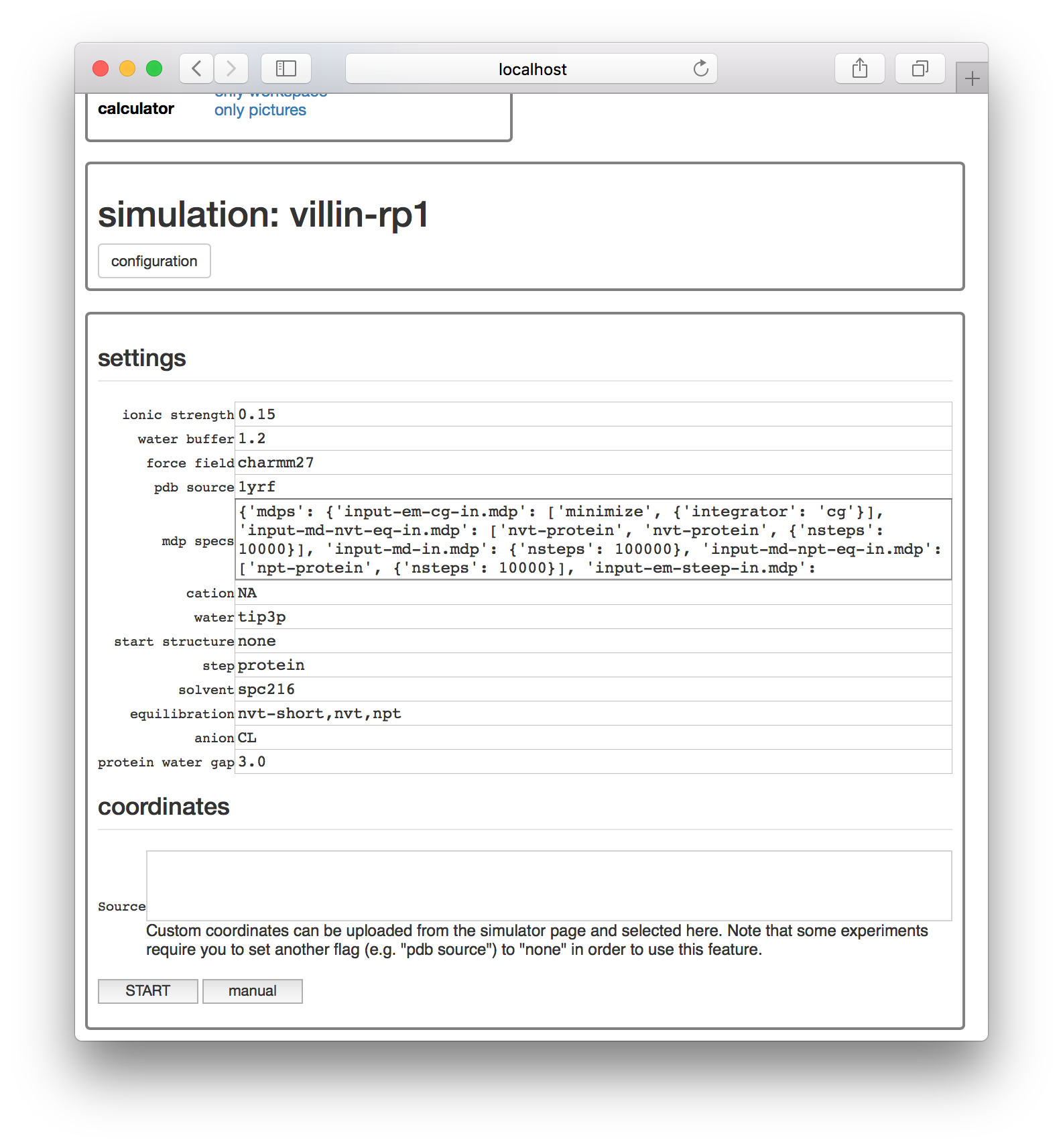
The “pdb source” parameter will download a fragment of villin headpiece from the protein databank according to its code 1yrf. If you set this value to none and upload a PDB structure on the main page, you could alternately select your structure from the “sources” list. This feature is necessary if you need to pre-process the structure. When you have reviewed the parameters, click the “start” button to launch the simulation.

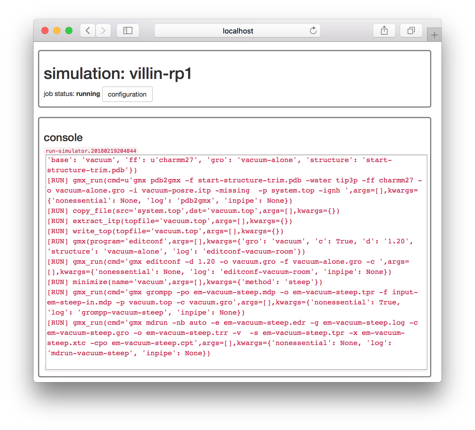
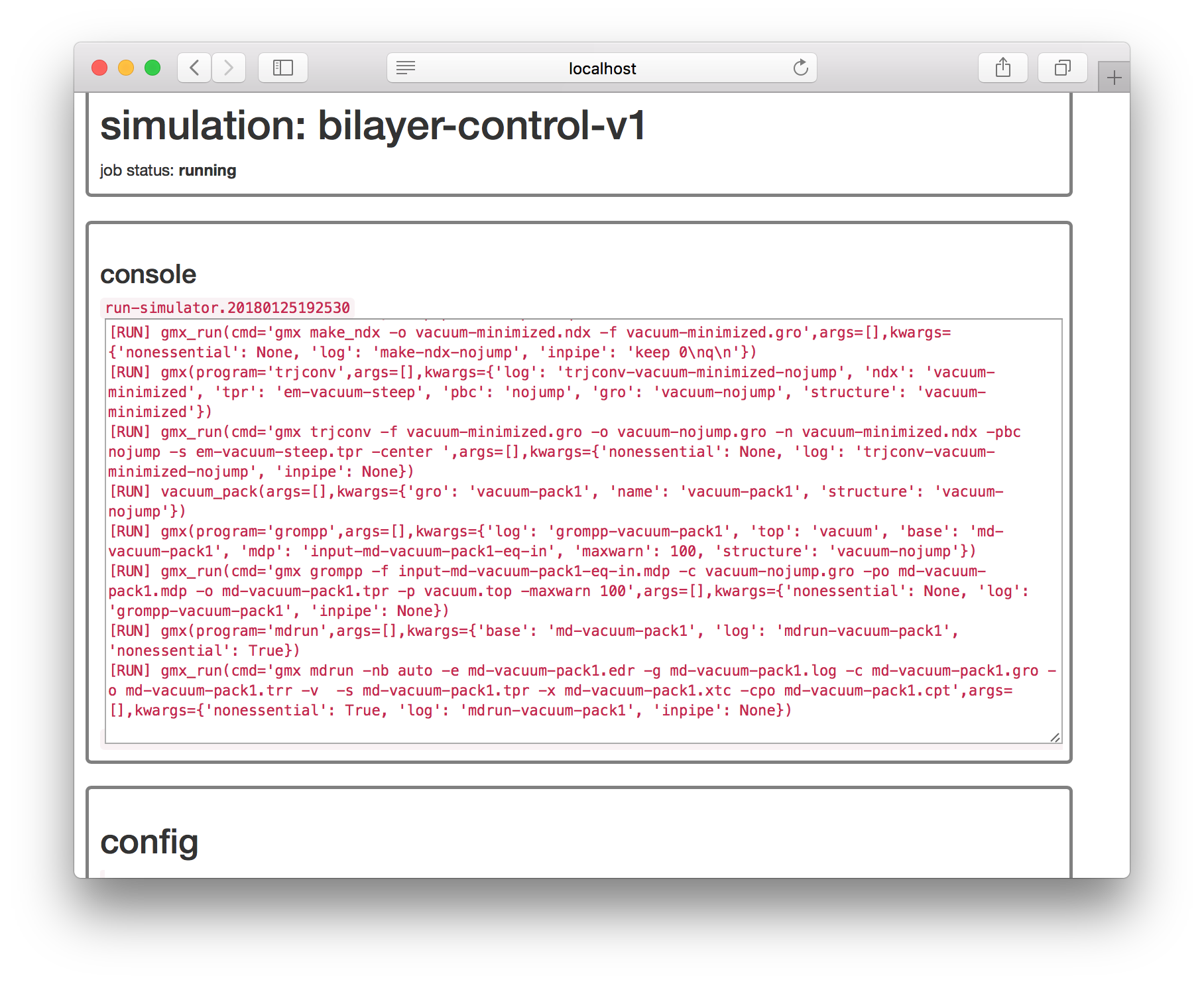
The next page will claim the simulation is “waiting” but if you refresh the page you should see a live console of its progress.

You can go back to the simulator page by clicking the toggle button on the first tile. There you should see that our job is in a small cluster of simulations.

Using custom structures

Earlier we mentioned that you might wish to use a custom starting structure. This is often necessary if the PDB structure contains multiple conformations, in which case you must edit the file to choose one. You may also perform homology modeling to add missing residues (note that we have experiments for this use-case, but they are not yet published).

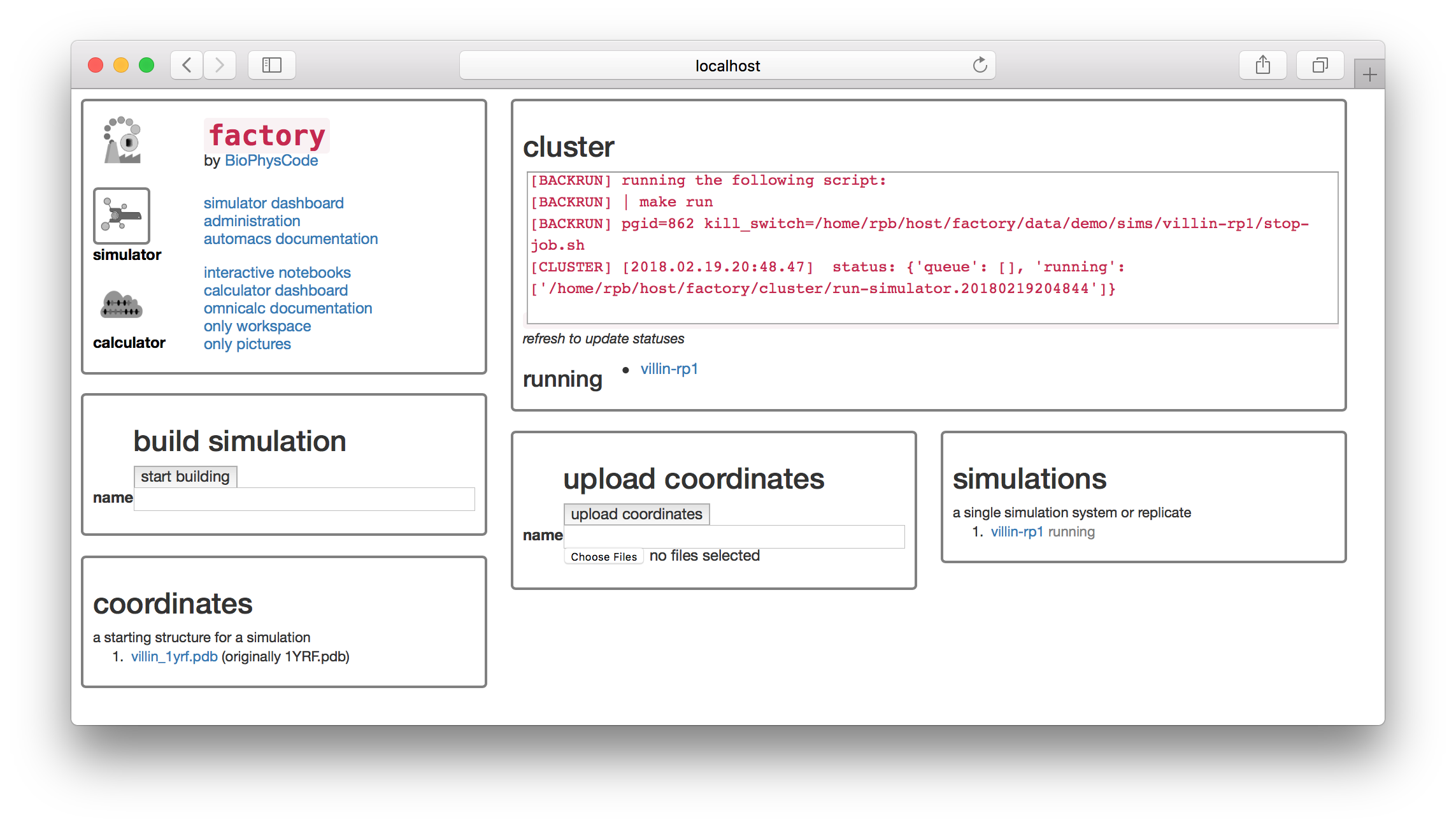
On the simulator page, select a name for your structure in the “upload coordinates” dialog. We choose villin-struct-v1 and then used the “Choose Files” button to select the 1YRF.pdb file which we downloaded manually from the PDB here. This is the same structure that AUTOMACS automatically downloaded before, but we are using it here for demonstration. After clicking “upload coordinates” you can see that there is a new entry in the “coordinates” tile.

To use these coordinates, start another simulation as before. On the settings page, change “pdb source” to “none” as shown in the image below. This tells AUTOMACS not to automatically downlad this from the PDB. Then, select villin-struct-v1.pdb from the “Source” list to use the structure.

Once you click “start” and return to the simulator page, you can see that both simulations are running.

Running an analysis

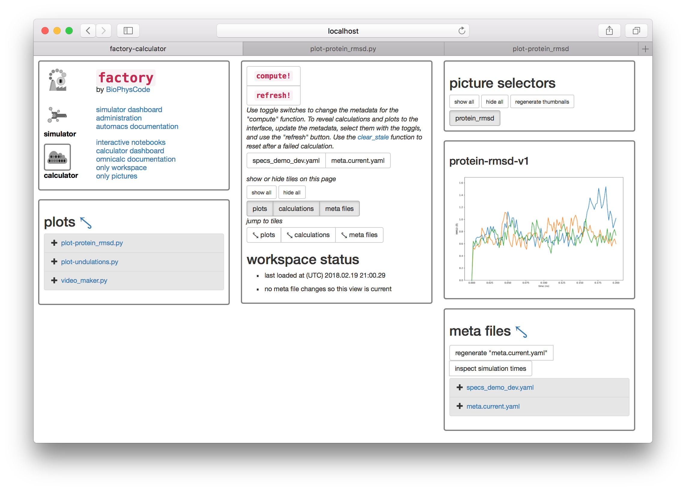
Once both simulations are complete we can analyze them. We will compute the protein root mean-squared deviation which is also described in the calculation guide. Click on the “calculator” toggle in the first tile.

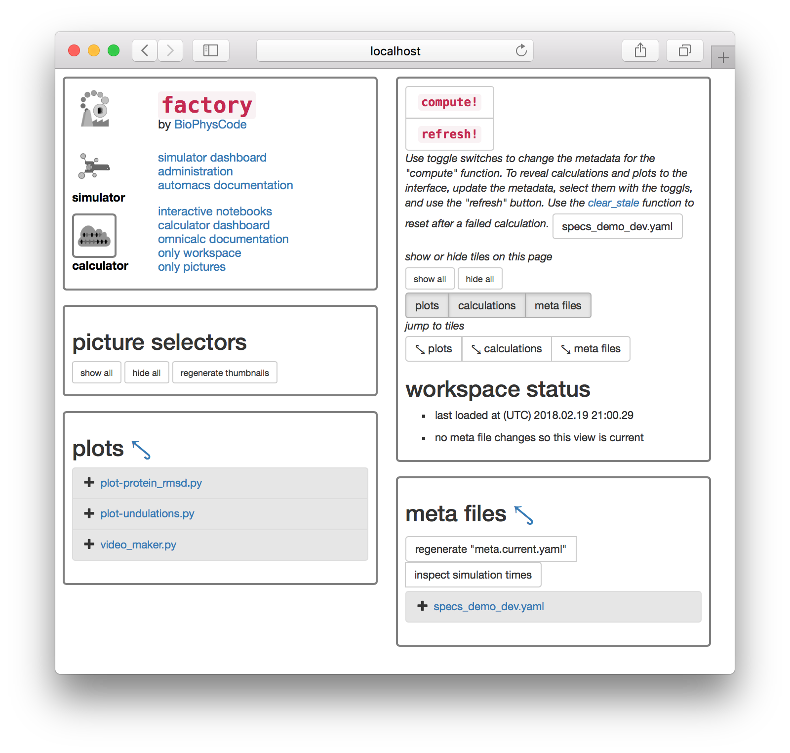
First we will generate the necessary metadata for our analysis. The following steps will make an example metadata file for you, but you are free to edit these by clicking on the entries in the “meta files” tile. At the top of this tile there is a button titled “regenerate ‘meta.current.yaml’”. When you click it, a file called meta.current.yaml will appear below. If you click on the link to the meta.current.yaml file you will visit an IPython notebook. The factory uses one port to serve the main factory pages and a separate port to run a notebook server for analysis. The notebook is pictured below. IPython supplies an editor.

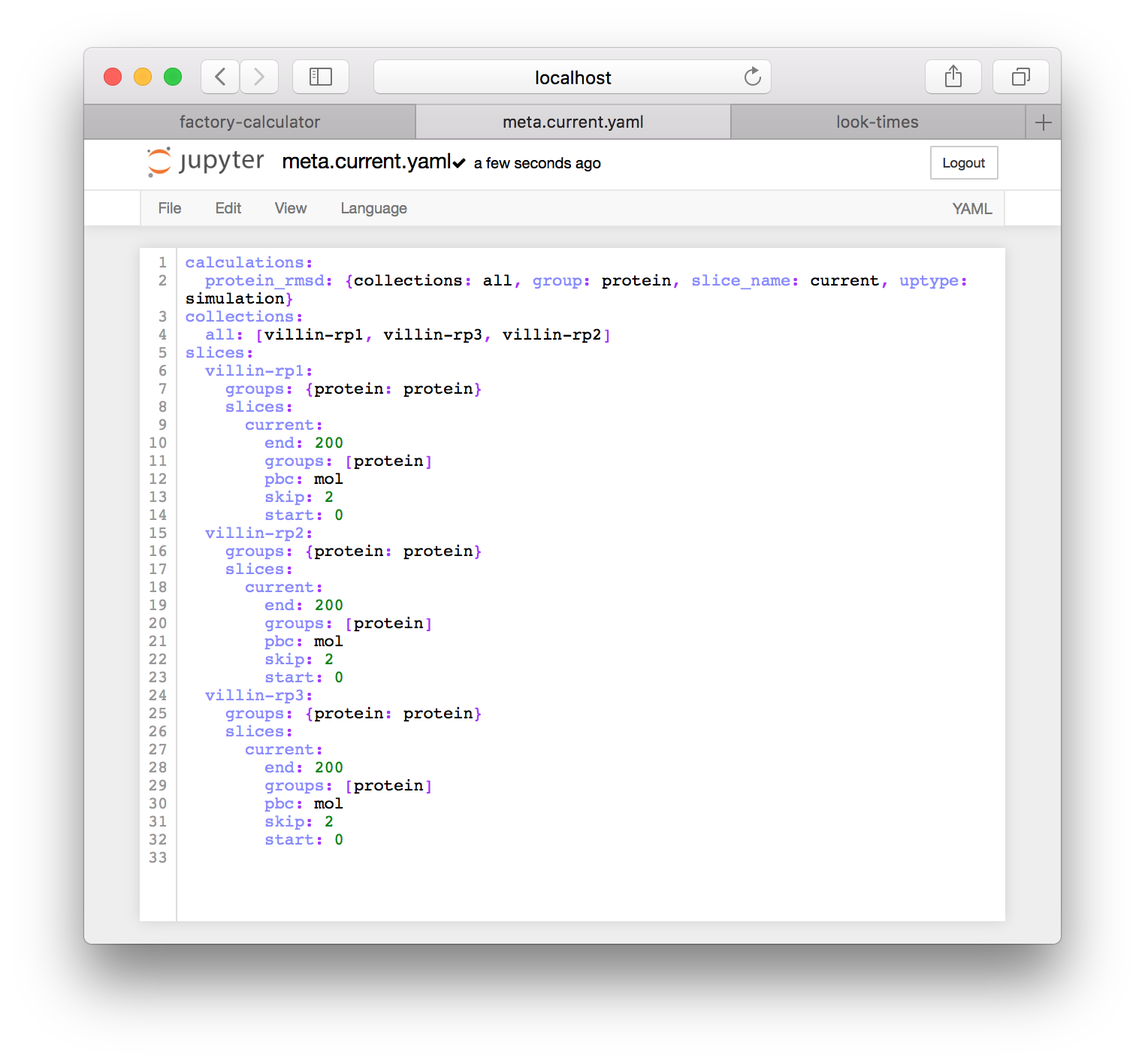
This notebook is written in the YAML format and was automatically generated by the “regenerate” button described above. You can always rename this copy by first clicking on the “interactive notebooks” link on the main page and then using the regenerate button again. It contains three entries. The collections list creates a single group called all for analyzing your simulations. The calculations list includes the default calculation called protein_rmsd which will be described below, and points the calculation code to the all collection and the samples described below. Those samples are requested in the slices list, which tells the calculator code how to make samples. In the example above, we are requesting a 200 picosecond (ps) trajectory, sampled every 2 picoseconds, with contents given by the selection command "protein".

Note that most simulations are set to run for a very short time, for demonstration. These simulations can be continued by running a local script called script-continue.sh which is written along with the data after the first run. Recall that simulations are stored in factory/data/demo/sims and this script should be found in the s01-protein step. After you continue your simulations, can you check the simulation time by returning to the main page and clicking “inspect simulation times”. This takes you to an IPython otebook with a single cell, which lists the various parts of a completed simulation. An example is provided below. This method is equivalent to running make look times from the omnicalc directory.

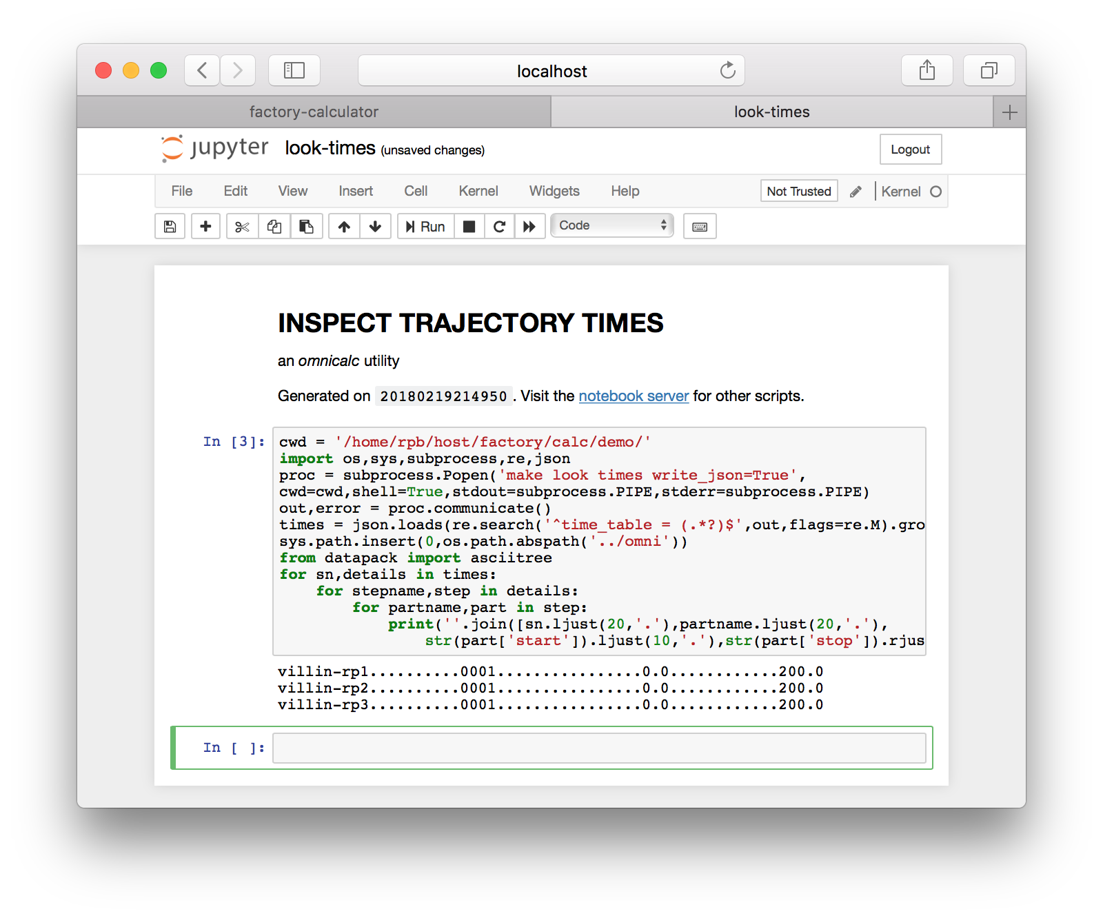
This page is useful for checking your simulations to see that they have accumulated enough time. Return to the main page.

Running the RMSD calculation

When we connected to this project, we cloned a calculations repository that includes protein_rmsd.py. You can inspect and edit that code by following the link on the “calculations” tile. Note that this tile might be missing, since omnicalc only identifies these calculations when it checks the metadata. To reveal the calculations tile, toggle meta.current.yaml and use the refresh button. The calculations tile will appear. Since our project already includes this code, and we have prepared the proper metadata, we are ready to run a calculation.

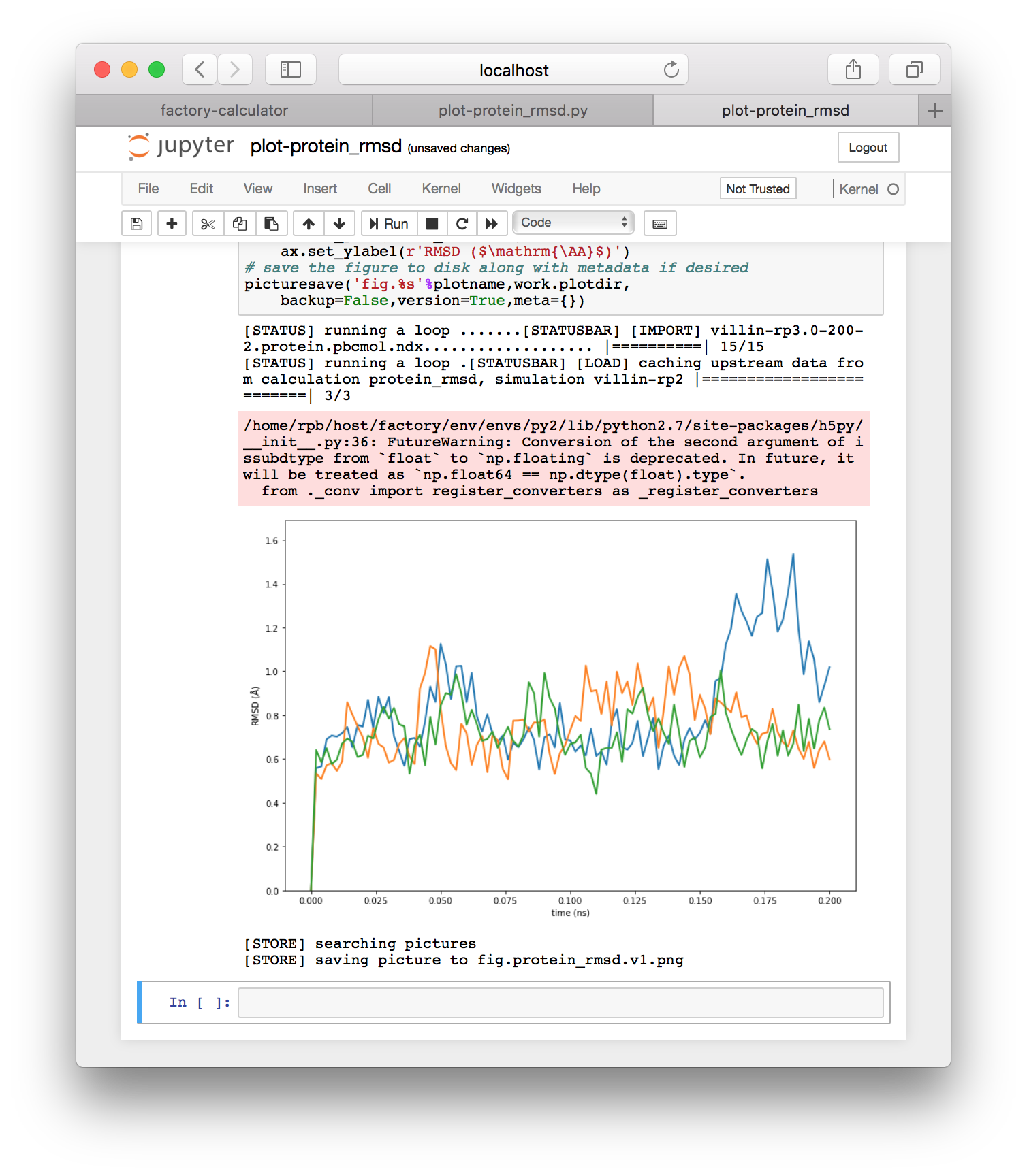
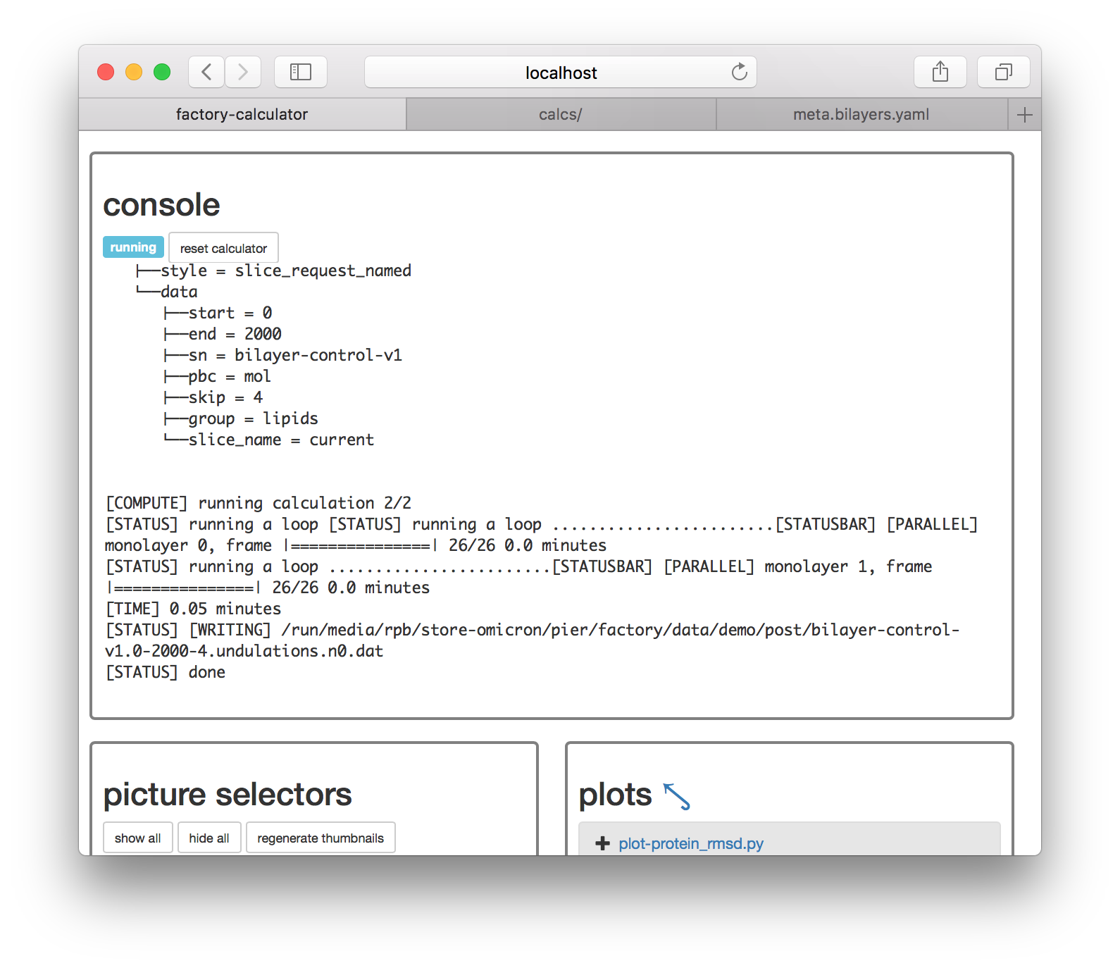
Select the meta.current.yaml toggle switch underneath the “compute!” button to tell the calculator you wish to run calculations from that metadata. Then, click “compute!” and you will see a console appear. If it resembles the following screenshot, then your calculation has been run successfully and written to disk.

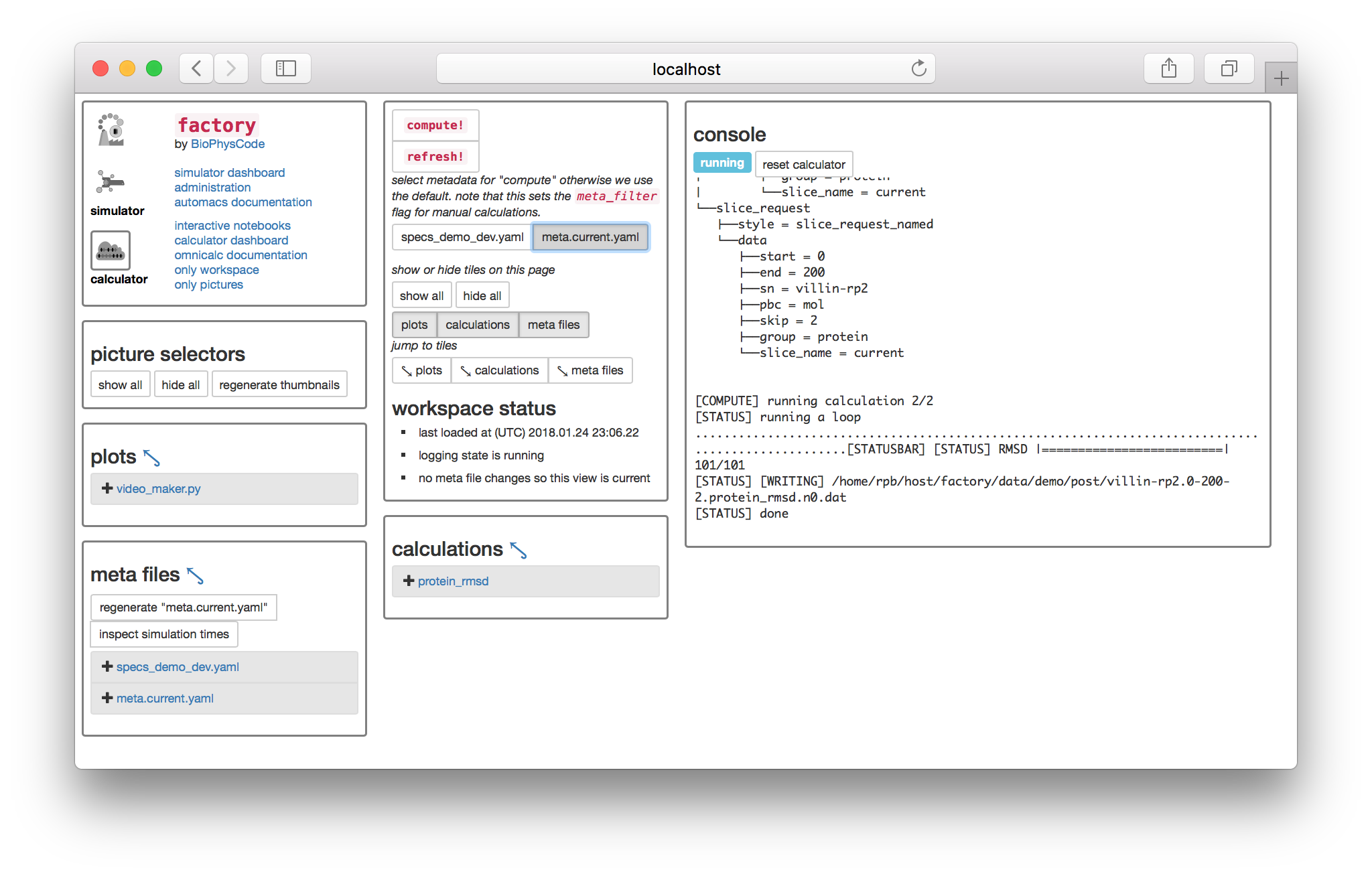
The console captures terminal output so it might appear somewhat confusing. The last line tells you that it wrote a file called villin-rp2.0-200-2.protein_rmsd.n0.dat. This file is the result of the protein_rmsd calculation, applied to the second replicate, called villin-rp2, using a slice generated from 0 through 200 ps, with a sampling rate of 2ps. The extra suffix n0 is used to index different calculation parameters which we do not wish to include in the filename, but since the RMSD calculation has none, it points to a single copy. Calculations are only run once. If you press the compute button again, it will notice the files on disk, which are located in the post-processing folder at factory/data/demo/post.

Plotting the protein RMSD

To plot our data, we will create a new plot script. Note that this is the same script that we used in the calculation guide. There should be a file in the “plots” tile called plot-rmsd.py. Clicking it will open the script in a separate tab for viewing.

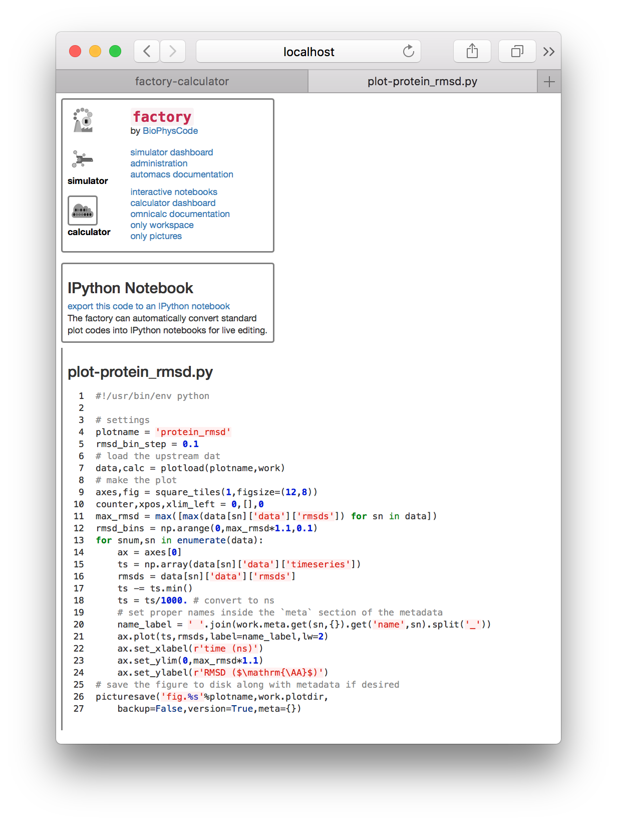
If you haven’t already, click “export this code to an IPython notebook” and a new link will appear. Clicking that link will take you to an IPython notebook that has been derived from the plot script.

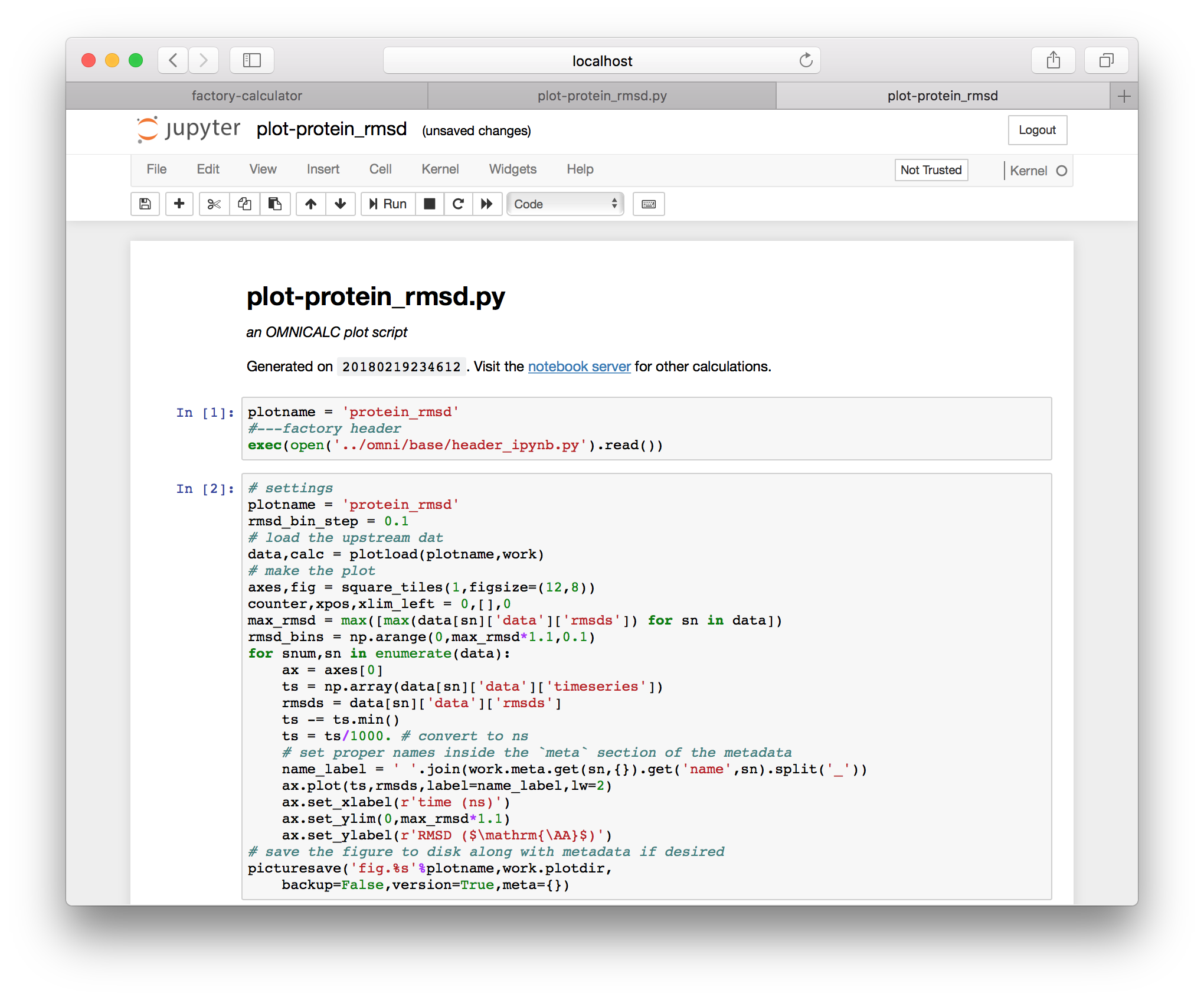
It can be useful to rename these if you make edits, and they can always be regenerated from the same underlying python script, which has been found in the calculations repository we specified above. If you run the cells from this plot (via shift+enter), you will generate the RMSD plot shown below.

Note that running the interactive script will also save the plot to the “plot spot” set earlier, at factory/data/demo/plot. Note that you can view, copy, or otherwise edit all IPython notebook files generated by the factory by clicking the “interactive notebooks” link on the navigation tile of either the simulator or calculator pages.

If you return to the calculator page by using the button in the first tile, you can use the “picture selectors” to view all of your analyses.

Summary. So far this walkthrough has shown you how to make an omnicalc project, run a short simulation, and run a basic analysis from code shared on github. The rest is up to you. You can write new calculation scripts similar to protein_rmsd.py in the calculations repository factory/calc/demo/calcs and make your own repository from this directory so you can share it with others. You can also write new plot scripts here, and these can be automatically converted into interactive notebooks for plotting and further analysis. You can also find your simulations at factory/demo/data/sims where they can be extended. The factory will let you re-sample and analyze the new simulations by using the “inspect times” or “regenerate ‘meta.current.yaml’” buttons. You can also make new metadata for different analyses.

Remember that all of the paths are controlled by the connection file at the beginning of the guide, and hence you can save the data wherever you like by choosing these paths carefully. In the next section we will show you how to run coarse-grained simulations, but this guide has covered the basics of the workflow.

Running coarse-grained simulations

In the second part of this review, we will run a coarse-grained simulation of a bilayer using the MARTINI force field. Since the procedure is very similar to the atomistic protein simulation, we will describe it with fewer images and more words.

To make a bilayer simulation, go to the simulator page, name a new simulation bilayer-control-v1, and click the “build simulation” button. Choose the all kickstarter followed by the bilayer_control_multiply experiment (recall that in the protein tutorial we choose the proteins kickstarter and the protein experiment). Once you have selected the experiment, you will visit the settings page. This experiment is somewhat more complicated than the protein experiment, because it has two separate parts. We are typically interested in the effects of proteins on a bilayer, so this simulation of a free bilayer could act as a starting substrate or a negative control, hence the name.

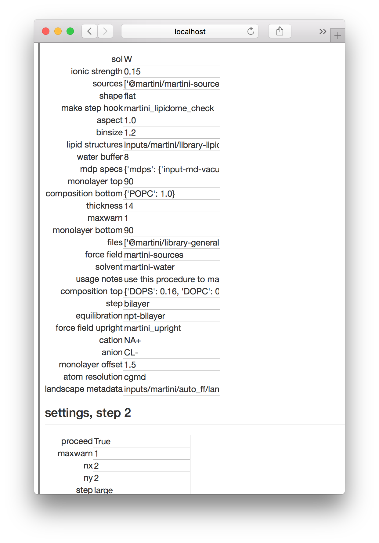
In the first step, we make a small coarse-grained bilayer and in the second step we “multiply” it by duplicating it in two directions to make a larger bilayer. The settings shown above include a dictionary that sets the composition, the thickness of the box before we add water (in nanometers) and the number of lipids in the top and bottom monolayers (that is, “monolayer top”, etc).

The second step tells automacs to make the bilayer four times as large by settting the “nx” and “ny” flags. Run the simulation and go get some coffee. It should take about ten minutes. Remember to refresh the page if it says that the simulation is “waiting” or return to the simulator page while it runs.

Once the simulation is complete, go to the calculator page. Recall that in the protein simulation above we had automatically created a file called meta.current.yaml which checked the simulation times and prepared a request to make “slices” of these trajectories for analysis. Since we are adding more simulations to this project, we will organize these metadata files more clearly.

First, we will rename meta.current.yaml to meta.proteins.yaml by clicking on “interactive notebooks” on the navigation tile, which is the first tile in the upper left. This opens up the IPython (Jupyter) notebeook server which works like a file manager. All metadata are stored in the specs folder. To rename a file, click on the corresponding checkbox and use the “rename” button above. Since we are adding coarse-grained simulations to a project that started with atomistic proteins, it is important to keep these metadata separate. The toggle switches on the calculator page allow you to select different sets of metadata before running either “compute” or “refresh” operations. This can be useful for managing your workflow.

Once you have renamed the protein metadata, return to the calculation page and refresh the page (not by hitting the “refresh” button, but by refreshing in the browser). You should see that the meta files reflect the renamed files in your calcs/specs folder. Note that there may be extraneous metadata files there too, particularly since we cloned a calculations repository which might be used for multiple projects. In this case you should ignore the file called meta.plots.video_maker.yaml.

Now we will construct metadata to analyze the bilayer simulation. First we need to see how long it ran. On the calculator page, click “inspect simulation times” and run the only cell in the notebook which opens in a new tab. We find that the bilayer control has run for 2,000 picoseconds.

Return to the IPython notebook server. If you left it open in another tab, use that, but otherwise you can get there with the “interactive notebooks” link on the navigation tile of the main page. Go to the specs folder and use the “new” button in the upper right to make a new text file. This will open a blank text file. Add the following text to the file and rename it to meta.bilayers.yaml by clicking the name at the top of the page.

variables:
  selectors:
    resnames_lipid: ['DOPC','DOPS','POP2','POPC']
    lipid_selection: (resname DOPC or resname DOPS or resname POP2 or resname POPC)
collections:
  cgmd_bilayers: [bilayer-control-v1]
slices:
  bilayer-control-v1:
    groups:
      lipids: +selectors/lipid_selection
    slices:
      current:
        end: 2000
        groups: [lipids]
        pbc: mol
        skip: 4
        start: 0
calculations:
  lipid_abstractor:
    ignore: False
    slice_name: current
    group: lipids
    collections: cgmd_bilayers
    specs:
      selector:
        resnames: +selectors/resnames_lipid
        type: com
      separator: 
        cluster: True
        lipid_tip: "name PO4"
  undulations: 
    collections: cgmd_bilayers
    group: lipids
    slice_name: current
    uptype: simulation
    specs:
      upstream: lipid_abstractor
      grid_spacing: 0.5
plots:
  undulations:
    autoplot: True
    collections: cgmd_bilayers
    calculation: undulations
    slice: current

The prepared file should resemble the following screenshot.

This metadata has several sections.

variables provides data which can be used elsewhere using a path syntax such as +selectors/lipid_selection
collections tells the caclulator which simulations to analyze
slices tells the calculator to sample the 2,000 ps trajectory (recall that we found the end time from the “inspect simulation times” button)
calculations tells the factory to run two calculations: lipid_abstractor and undulations, and connects the calculations to the slices (current), group (lipids), and simulations (the collection cgmd_bilayers)
plots tells the factory how to run the plot script, which is found at plot-undulations.py

Return to the calculator page, which might still be open in another tab. The metadata we have just created has not yet been recognized by the code. Underneath the compute button there are toggles which we can use to select new metadata. Click the toggle titled meta.bilayers.yaml and then click the “refresh” button. You should notice that some new calculations appear, specifically the lipid_abstractor and undulations codes mentioned above. The factory noticed these calculations because they were found in the calculations section of the metadata we prepared. You can click the links to edit the code.

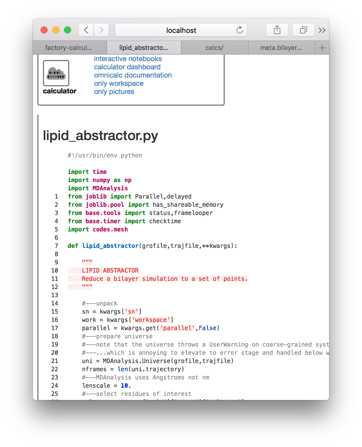
This code is worth reading later. It relies on a modle at calcs/codes/mesh.py which generates are regular mesh from the lipid centers of mass. These are computed first by lipid_abstractor.py, saved to disk, and then interpreted by undulations.py. Having prepared the metadata correctly, we can now use the “compute” button. The slices are made with the GROMACS gmx trjconv utility and calculations are logged to the console.

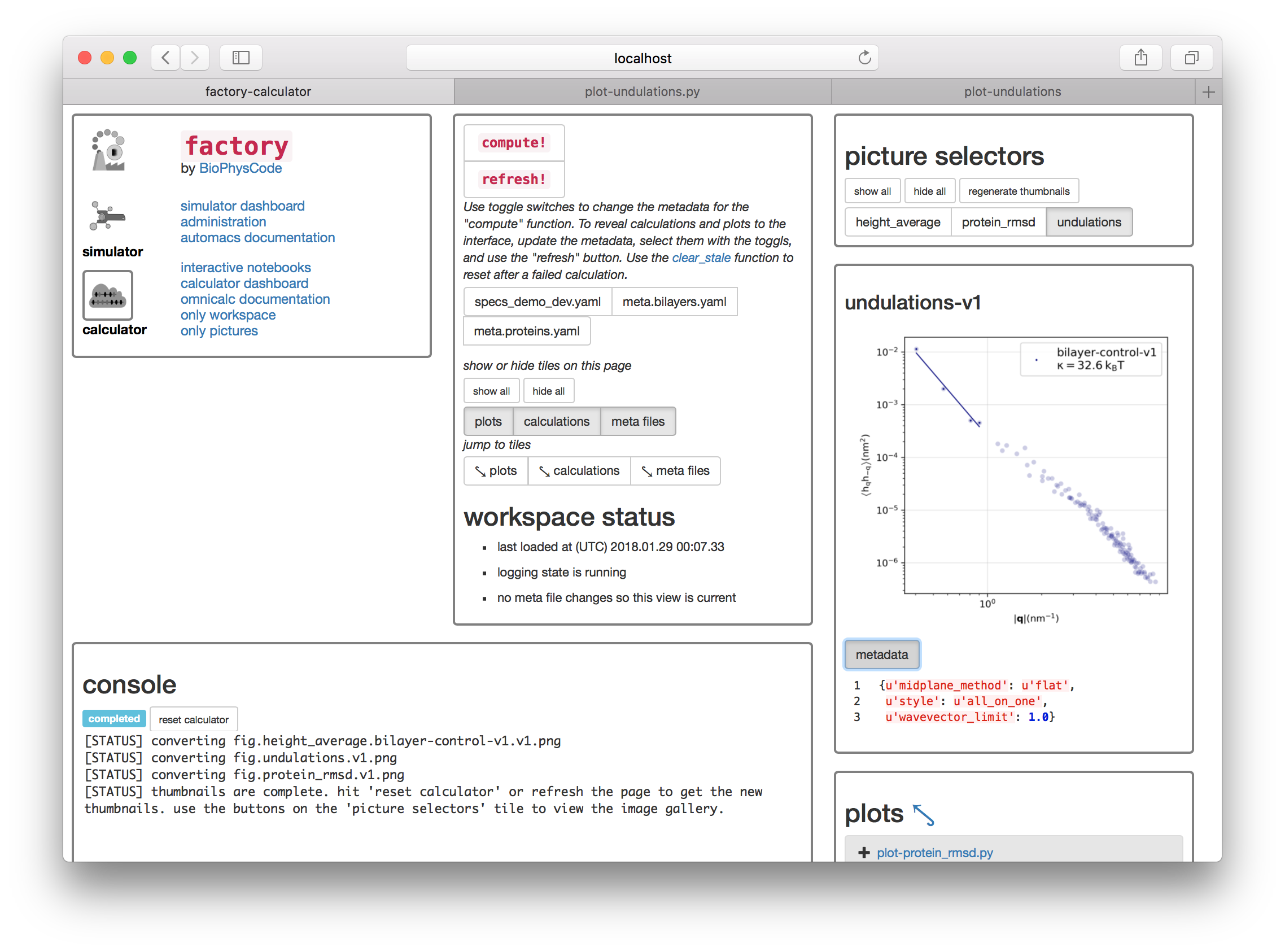
Now that the calculation is completed we can plot the results. Click on the plot-undulations.py link on the calculator page. On the following page, use the “export” link to turn this python script (located at calcs/plot-undulations.py) into an interactive notebook. The notebook will be written to calcs/plot-undulations.ipynb will be accessible later from the “interactive notebooks” link.

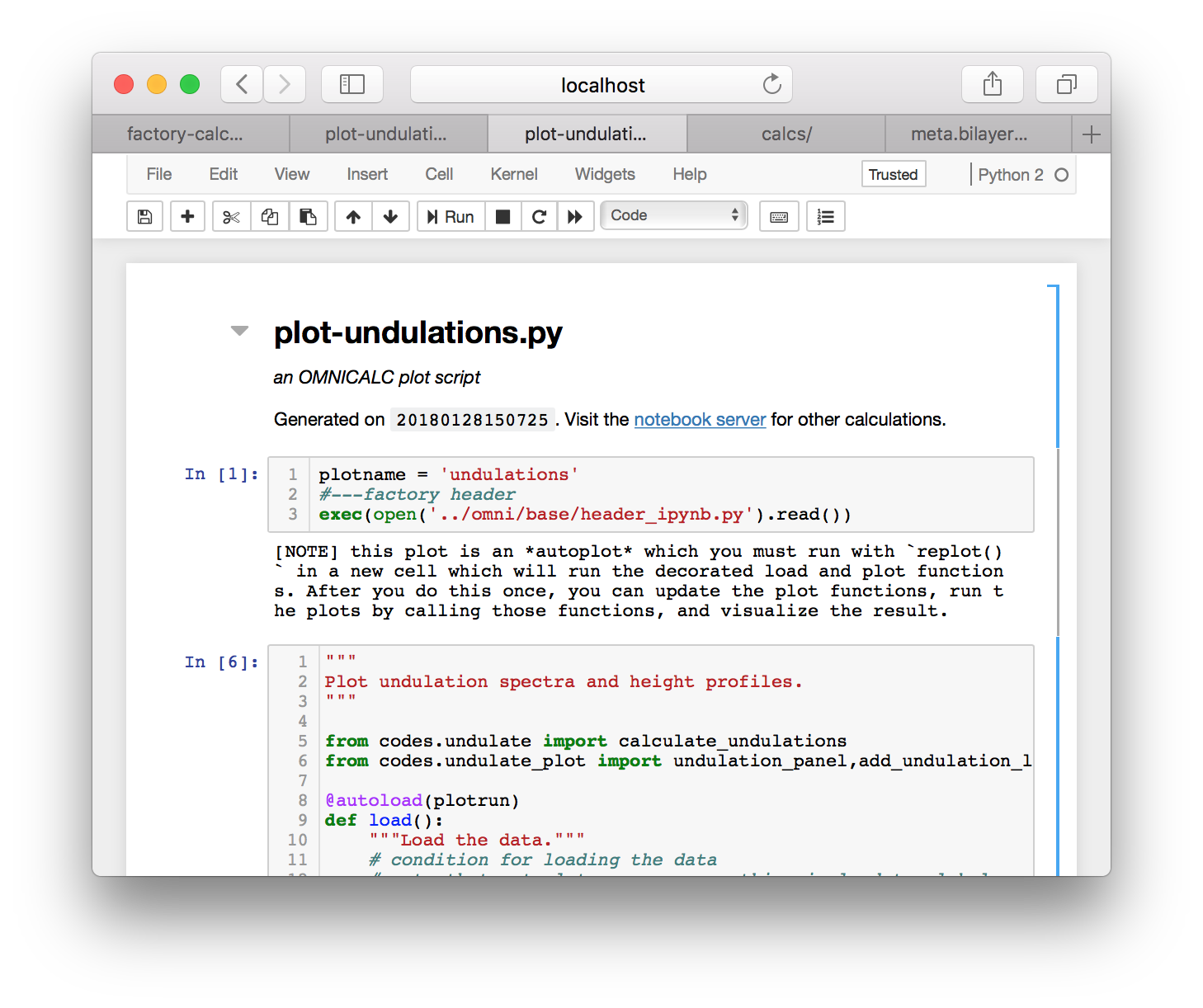
After you run the first cell, the code warns you that this plot script is an “autoplot” which means that we must run the replot() function at the end to executing the functions. The autoplot scheme is documented in further detail in a separate tutorial. Running each cell, followed by replot() will produce an undulation spectrum and an image of the average height profile of the bilayer. These plots are also saved to factory/data/demo/plot for later.

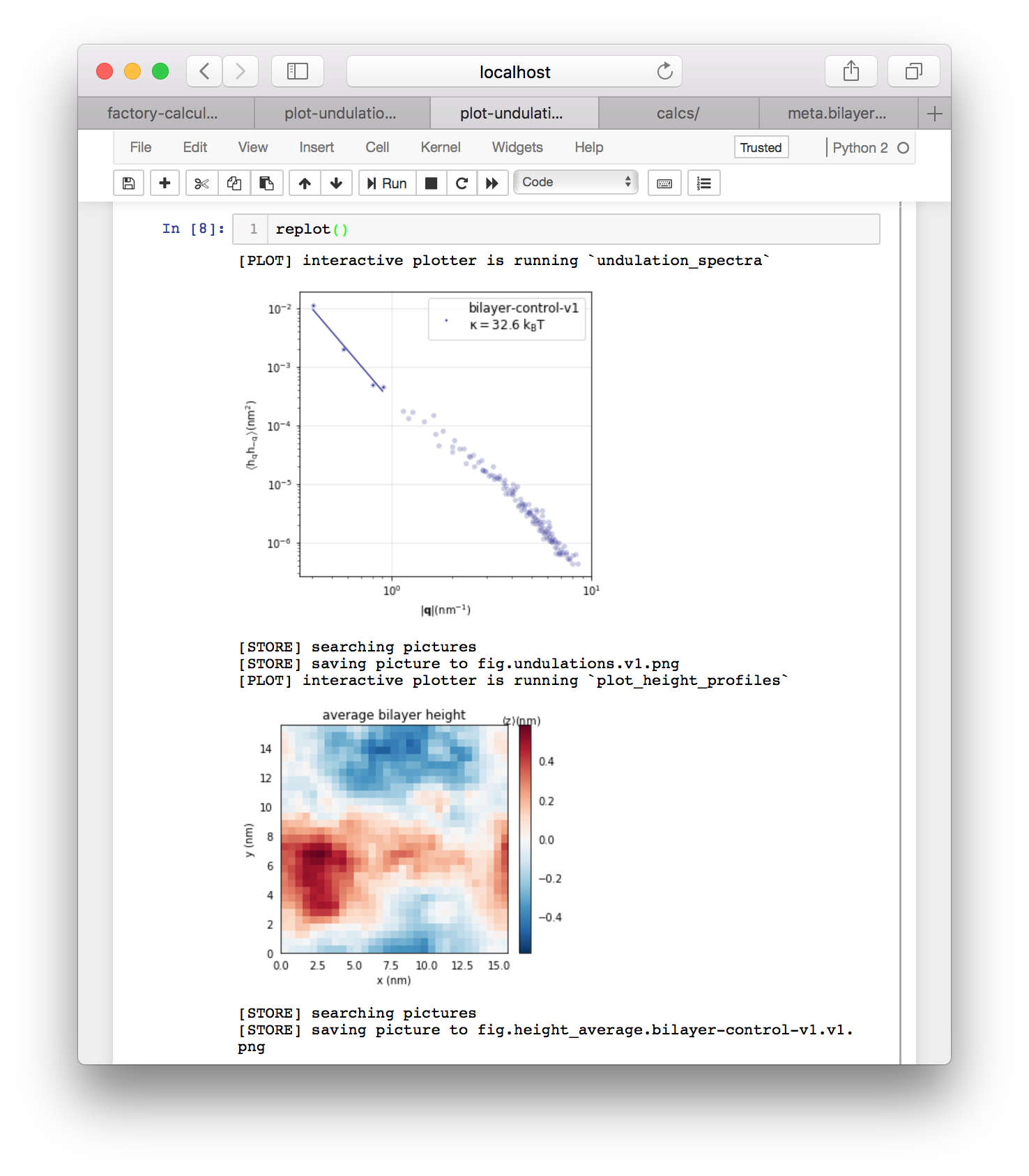
If you return to the calculator page and click “regenerate thumbnails” in the “picture selectors” tile then the undulations toggle will appear in the same tile. You can use these toggles to view the plots of your data. You can also click the metadata toggle to see relevant information about the plot.

Rendering videos

If you have VMD installed you can render a video of the protein simulations. Click the video_maker.py entry on the plots list. This opens a page showing the original code shown below.

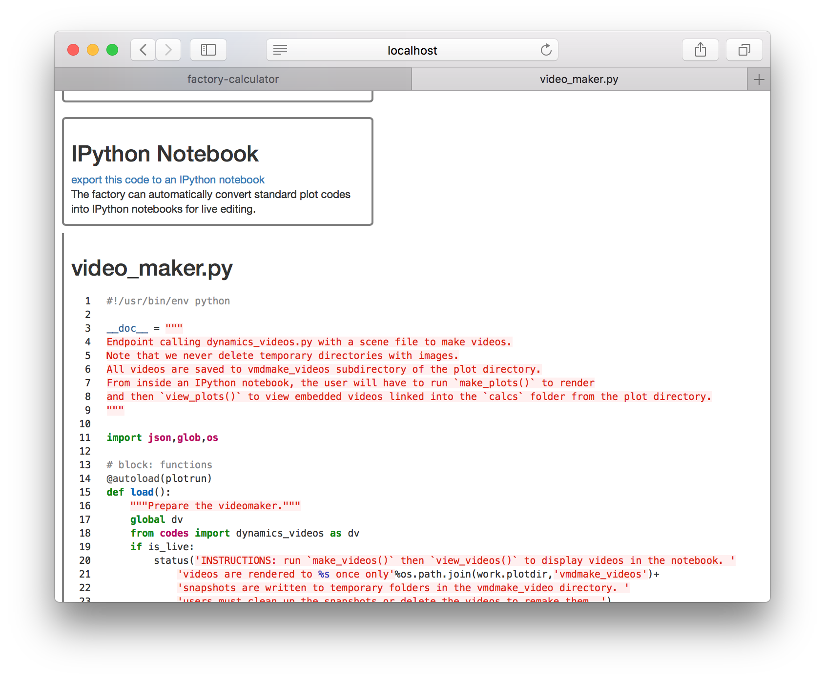
Click the link titled “export this code to an IPython notebook” to make an interactive version, then click the resulting link to open the notebook.

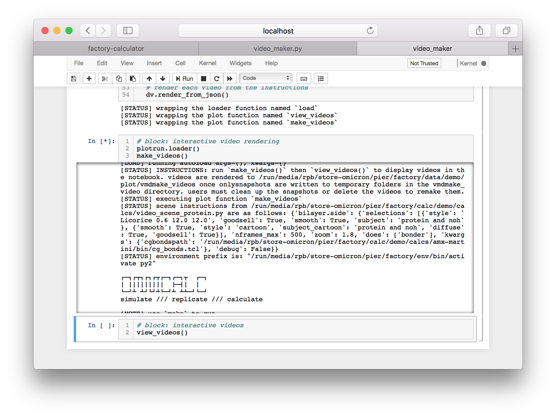
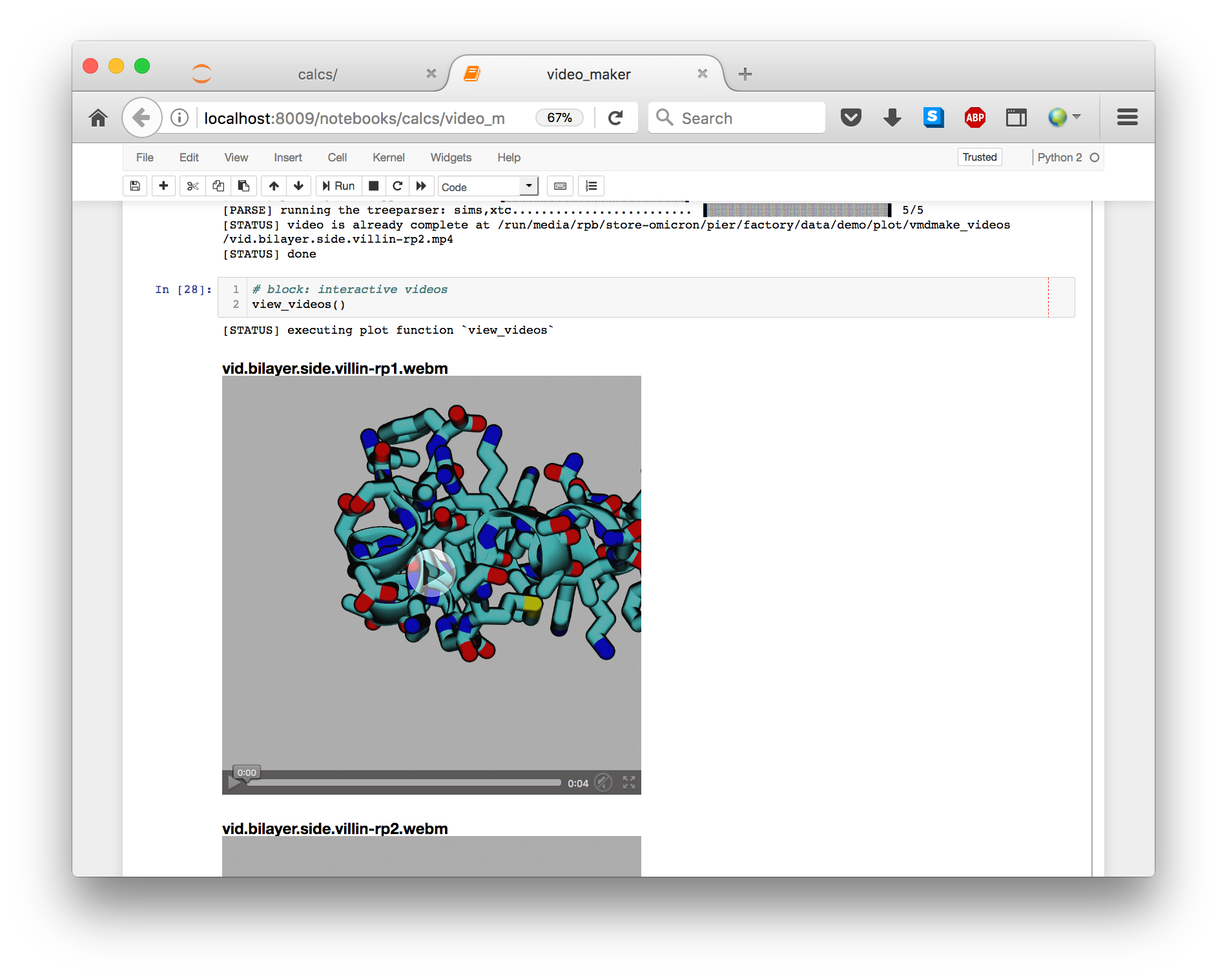
Running the cells in this notebook will make the videos in a subdirectory of your plot folder. The features of the video are controlled in a separate file called video_scene_protein.py. The final cell will link the videos into the script so you can view them.

Concluding remarks

The factory workflow follows the patterns described above. First you run a simulation using an automacs “experiment”. Then, you write or retrieve a calculation function and carefully prepare metadata to link calculations to simulations. You tell the factory to use this metadata to analyze the simulations. Once they are ready, you run an interactive plot script to visualize them.

All of the operations that occur on the graphical interface have command-line equivalents and are covered in the omnicalc and automacs documentation.