BioPhysCode is a collection of three open-source biophysical simulation analysis tools developed jointly by Ryan Bradley, Joe Jordan, and David Slochower during their study at the University of Pennsylvania under the supervision of Ravi Radhakrishnan. It is currently under active development by Ryan and Joe.

Our goal is to provide all of our simulation and analysis tools to the larger research community. Each code works independently, however they are designed as a single, coherent framework so you can use them together to create novel, scalable biophysics experiments based on the popular GROMACS integrator. Contact the authors if you have questions, or open an issue on the github pages listed below.

We recommend starting with either the quickstart guide or the list of validated codes.

FACTORY
a flexible framework for building and analyzing molecular simulation data
◾ source from github
◾ contact the authors for instructions

AUTOMACS reproducible, extensible, shareable simulation protocols
◾ source from github
◾ online documentation

OMNICALC
transparent analysis pipeline for interpreting biophysical simulations
◾ source from github
◾ online documentation

Quickstart guide

Use cases

The following is the quickstart guide for BioPhysCode, which consists of a simulation package called automacs, a calculation package called omnicalc, and an interface called factory. This guide will cover the following use-cases.

1. Install a factory. The factory is primarily used to organize different calculation “projects” by cloning omnicalc and managing the paths to your data. It also manages a virtual environment which is required for running calculations, creating complex simulations with automacs, and serving the web-based interface. We recommend starting with the factory, which takes less than three minutes to install on most machines.
2. Make a standalone simulation with automacs according to a stock “experiment”. The authors provide many different simulation experiments, but the most common experiments will make an atomistic protein system (Joe’s favorite use-case) or a coarse-grained protein-membrane system (Ryan’s favorite use-case). This is best for users who are comfortable using the terminal and want to quickly generate new simulations.
3. Analyze preexisting simulation data from GROMACS, NAMD, or even custom mesoscale membrane simulations. This use-case is ideal for users who wish to use our analysis codes on simulations they have already created.
4. Run and analyze simulations in a single pipeline which can be served over a web-based interface. This is the most scalable use-case, and is best for users who wish to run many simulations and calculations that are already available in automacs and omnicalc.
5. Set up a factory inside a docker to either test the code, reproduce a specific use-case from another user, or securely serve a factory over the internet. Docker is effectively a sandbox which provides more control over the software environment and a secure way to serve many web interfaces from one machine. Additionally, the dockerfiles we provide can be used as a blueprint for building the software environment for a workstation you wish to use to run simulations outside of the docker,

1. Install a factory

Install a factory to supply software for advanced automacs simulations, or to organize your analysis of pre-made simulations.

The factory code does three things.

1. It supplies a python virtual environment for analysis and more complicated model-building. A simulation of a protein in water only requires GROMACS, but bilayer construction also requires Python libraries like SciPy.
2. It organizes instances of omnicalc into “projects” each of which can be used to analyze a set of simulations.
3. It creates a graphical interface to run and analyze simulations over the web.

There are two ways to install the factory. Users with a healthy linux environment can perform a “simple” installation by downloading a copy of Miniconda and installing it with the commands below. Users who wish to run the factory in a Docker should use the instructions in the docker section below. We recommend the simple installation if at all possible — Docker is useful primarily as a web server and as a method for ensuring that you know exactly how to set up a new linux box in order to run the simple installation yourself. Note that in the following example, I have saved a copy of the Miniconda installer the factory folder after I cloned it.

git clone http://github.com/biophyscode/factory
cd factory
make help
make set species anaconda
# download Miniconda before the next step
make set anaconda_location=./Miniconda3-latest-Linux-x86_64.sh
make set automacs="http://github.com/biophyscode/automacs" 
make set omnicalc="http://github.com/biophyscode/omnicalc"
make setup

Setup should take about three minutes. The commands listed above were also given by the make help command so you don’t have to remember all of these steps next time. Note that make help will always be up to date, in the unlikely event that we change parts of the code. Once you build the factory, you can source the included environment from anywhere by running source factory/env/bin/activate py2 as long as you use the right path to the factory.

Anytime you set up an omnicalc project in the factory (see the analysis guide), all of its make commands will automatically source the factory environment before they run, so you don’t have to remember this step for analysis.

Automacs simulations can be run from anywhere, but you have to remember to source the python environment for complicated use cases, for example bilayer construction. I prefer to make a shortcut to the source command so I can call it from other locations easily by adding alias py2="source /home/username/factory/env/bin/activate py2" to my ~/.bashrc file so that I can run py2 before starting simulations.

2. Standalone AUTOMACS quickstart guide

Run an “automatic GROMACS” simulation of a coarse-grained protein on a bilayer.

Requirements. To complete these commands you will need a working copy of GROMACS available at the terminal. The bilayer builder depends on SciPy as well, which you can install yourself or install with the factory according to the factory guide above.

You can clone automacs and the associated modules with the following commands.

git clone http://github.com/biophyscode/automacs
cd automacs
make setup all
make gromacs_config home
make prep v

The final command lists all of the available simulation “experiments”. The make gromacs_config command can write an automacs configuration file to either your home directory or in the automacs root folder. This configuration file will help you load the necessary software on the cluster, or set the number of processors for the integrator. The v flag uses a verbose mode that includes tags and test dates. The colorful tags show the last time the tests were run, and serve as notes for the developers. The make prep v command lists three types of “experiments”. We’ve highlighted the multi-step experiments (called “metaruns”) in the image below.

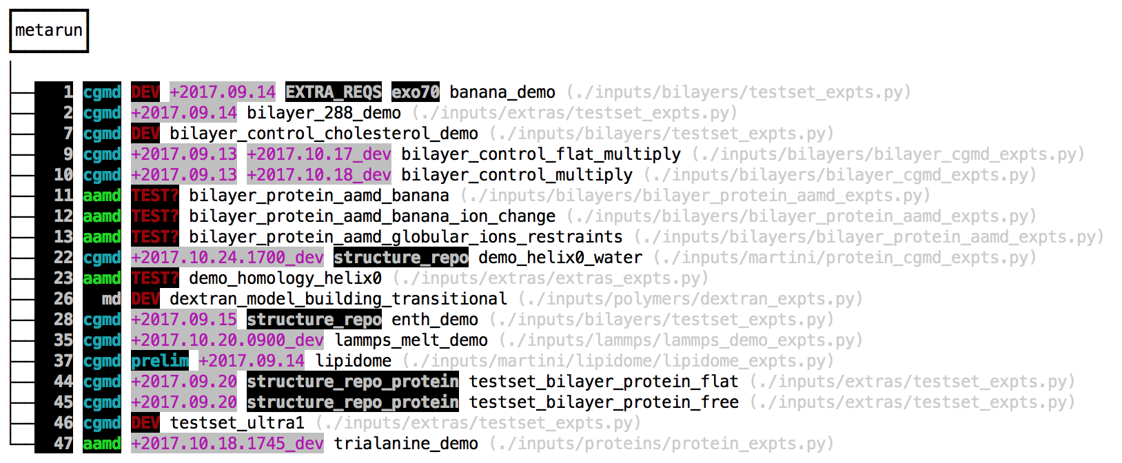
The make setup all command tells automacs to download independent repositories containing different experiments. You can also make your own modular repositories and load them into automacs. The default modules are loaded by make setup which can request one of several “kickstarters” that pull down several modules from github. The all kickstart is a good place to start. The instructions to run these experiments are found in the grey paths listed beside them. Because automacs uses “kickstarters” to load extra modules from github, it automatically detects any file that matches *_expts.py and parses it for experiments, so your list of experiments might be different.

The easiest way to run an experiment is to use the following command.

make go bilayer_control_flat_multiply clean back

The optional clean flag erases the previous simulation data in this copy of automacs, so be careful! This option is useful when adjusting parameters and restarting the simulation. The optional back flag runs the simulation in the background. Automacs will prepare the necessary python scripts and run them for you. Note that the experiments listed above are composed of other modular experiments (which we call “runs”) hence the sequence is called a “metarun”. Automacs is designed to be modular so that different runs can be reused in other contexts. For example, you can build a bilayer, duplicate it in several directions, and then attach a protein to it by calling on these individual steps inside of the experiment file. This minimizes repetition in our codes.

Most users prefer to start with one of the following examples.

1. protein will simulate a small protein in a water box. This is available with a smaller kickstarter invoked via make setup protein after you clone automacs.
2. testset_protein_bilayer_flat will create a coarse-grained bilayer and attach a small helix to it. This requires the make setup all kickstarter after cloning, and also requires SciPy, provided by the factory or available at your terminal.

Both experiments obviously require a working copy of gromacs. Other validated experiments are listed at the end of this guide. Users who wish to run coarse-grained simulations should check out the detailed coarse-grained bilayer guide for a more thorough walkthrough. The protein experiment also leads the walkthrough that helps to explain the experiment file, which includes all of the parameters necesssary to design the simulation.

3. Analyzing simulations

Automacs will replicate a simulation but you may wish to repeat or modify a calculation on a pre-existing dataset. In this section we will outline this use-case, in which we “reproduce a calculation.” The core calculation code (called “omnicalc”) can be used directly, but it is more convenient to manage your analysis pipeline with an instance of the factory. It will ensure that you have the right python libraries and it will tell omnicalc where to find your data.

This use-case assumes that you have already run a simulation and created a structure and trajectory file for analysis. The pipeline documentation below will describe how you can use the factory to simulate and analyze the data more seamlessly, but oftentimes users have already generated data that they wish to analyze, hence this section represents the simplest way to run a calculation.

Start by making a factory. Once it’s ready, you should write a “connection” file to a subfolder called connections. Note that whenever we use the location of a code, i.e. “make a subfolder in the factory,” we are referring to the place on disk where you cloned it. Choose a name for your project. This name will be used in several locations, so choose carefully! We are calling this one “proteins”, since we might include lots of simulations of different proteins.

proteins:
  site: site/PROJECT_NAME  
  calc: calc/PROJECT_NAME
  repo: calc/PROJECT_NAME/calcs
  database: data/PROJECT_NAME/db.factory.sqlite3
  simulation_spot: data/PROJECT_NAME/sims
  # place to store post-processing data
  post_spot: /home/username/data-post/
  # place to store the resulting plots
  plot_spot: data/PROJECT_NAME/plot
  spots:
    sims:
      namer: "lambda name,spot=None: name"
      route_to_data: /home/username/external_disk
      spot_directory: protein_activation_project
      regexes: # use regular expressions
        top: '(.+)' # regex to match simulation names
        step: '(production)' # all trajectories are in a subfolder
        part:
          xtc: 'md\.part([0-9]{4})\.xtc'
          trr: 'md\.part([0-9]{4})\.trr'
          edr: 'md\.part([0-9]{4})\.edr'
          tpr: 'md\.part([0-9]{4})\.tpr'
          structure: '(system|system-input|structure)\.(gro|pdb)'

Save the above text to factory/connections/protein_connections.yaml and then run the following command from the root directory.

make connect proteins

When it’s complete, your omnicalc project will be set up at factory/calc/proteins. We will run all of our commands from this folder. The repo flag points to folder where we will store our calculation codes. This folder will hold an independent git repository which you may later share with other users who can use the repo flag to clone your calculations over the web or secure shell. The calculations will be stored at factory/calc/proteins/calcs. At the end of this guide we will explain how to share your calculations repository.

Importing simulation data

The “omnicalc” code is designed to read simulations created in the corresponding “automacs” code, however it is easy to use the connection file above to point to GROMACS data that you’ve already generated. There is only one requirement: each simulation must have its own folder, and the trajectory “parts” must be in a subfolder. GROMACS generates several different output files typically prefixed according to the deffnm flag to the mdrun program. The spots section of the connection file can be used to point to multiple folders that contain source data. Each of these is a “spot” with its own path. In the example above, we have a single spot called sims which points to simulation folders at /home/username/external_disk/protein_activation_project. The remainder of the connection file tells omnicalc how to find the various trajectory (xtc and trr), energy (edr), and structure (gro or pdb) files using regular expressions. The top key has a generic regular expression '(.+)' that will match any simulation name, however you can use it to match certain folder names. If you used deffnm correctly, then the connection file above will help you locate trajectory files with paths like /home/username/external_disk/protein_activation_project/wild_type_rep1/production/md.part0009.xtc. The default GROMACS naming scheme used in the connection file will tell omnicalc to look for an arbitrary number of sequential files. We require energy (edr) files, run input files (tpr), and trajectory files at a minimum. We derive the timestamps from the energy files (because this is much faster than reading the trajectory data) in order to figure out how to stitch together many trajectory files for analysis.

Once you have prepared a connection file, run the following commands.

make connect proteins
make run proteins

The first command sets up an omnicalc instance and creates a calculation repository. The second command runs the graphical user interface (GUI) in the background at http://localhost:8000. Check out the single pipeline quickstart guide if you want to run simulations with this interface.

Running some simple calculations

In this step we will compute the root mean-squared deviation (RMSD) of a protein. This requires two new files: a “metadata” file to tell omnicalc which simulations to analyze, and a calculation file to analyze the resulting trajectory “slice”. We choose to store metadata in the YAML format because it’s easy to read. Make sure you start from the omnicalc folder at factory/calc/proteins. Save the file to calcs/specs/meta.yaml. Note that all of the files in the specs folder should be YAML. Later, you can use these files to fine-tune your analyses.

collections:
  one: [wild_type_rep1,]
slices:
  wild_type_rep1:
    groups: {'protein_selection':'protein'}
    slice:
      short: 
        {'start':10000,'end':20000,'skip':20,
          'pbc':'mol','groups':['protein']}
      long: 
        {'start':10000,'end':110000,'skip':200,
          'pbc':'mol','groups':['protein']}
calculations:
  protein_rmsd:
    slice_name: long
    group: protein_selection
    collections: one

The metadata above tells omnicalc to do several things. First, we define a “collection” of simulations to analyze. In the example above, we only have one simulation called wild_type_rep1. According to the connection file, omnicalc will expect to find trajectory files for this simulation at e.g. /home/username/external_disk/protein_activation_project/wild_type_rep1/production/md.part0009.xtc. Note that the simulation name matches the top regex in the connection file, while its subfolder matches the step regex and hence must be called production. This folder should contain all of the associated energy, run input, and trajectory files.

The second section of the metadata is called slices and tells omnicalc which part of the trajectory to use. In this case, we have requested a “slice” (i.e. a sample of our trajectory) from 10-110 ns with an interval of 200 ps (note that GROMACS uses picoseconds as the default time interval). The group named protein_selection uses the MDAnalysis package to select parts of your simulation, in this case the atoms returned by a CHARMM-style selection command 'protein'.

The next section, calculations tells omnicalc how to analyze this trajectory. In a moment we will write the calculation code to calcs/protein_rmsd.py, but for now, you should note that the calculation dictionary asks for the slice called long by its name, referring to the corresponding entry in the slices dictionary for this simulation. When we execute the calculation, omnicalc will try to find a trajectory slice that matches the one requested in the slices dictionary. If it doesn’t exist, GROMACS will make it automatically and save it to the post_spot directory set in the connection file for future use. It will also save the result of the analysis to this folder. Once all of the slices are ready, they will be individually sent to the calculation function.

To run the protein_rmsd calculation specified in the metadata, omnicalc will look for calcs/protein_rmsd.py. Save the following code to that location.

#!/usr/bin/python

from numpy import *
import MDAnalysis
from base.tools import status

def protein_rmsd(structure,trajectory,**kwargs):
    """Compute the RMSD of a protein."""
    work = kwargs['workspace']
    uni = MDAnalysis.Universe(structure,trajectory)
    nframes = len(uni.trajectory)
    protein = uni.select_atoms('protein and name CA')
    # reference frame
    uni.trajectory[0]
    r0 = protein.positions
    r0 -= mean(r0,axis=0)
    # collect coordinates
    nframes = len(uni.trajectory)
    coords,times = [],[]
    for fr in range(0,nframes):
        uni.trajectory[fr]
        r1 = protein.positions
        coords.append(r1)
        times.append(uni.trajectory.time)
    # simple RMSD code
    rmsds = []
    for fr in range(nframes):
        status('RMSD',i=fr,looplen=nframes)
        r1 = coords[fr]
        r1 -= mean(r1,axis=0)
        U,s,Vt = linalg.svd(dot(r0.T,r1))
        signer = identity(3)
        signer[2,2] = sign(linalg.det(dot(Vt.T,U)))
        RM = dot(dot(U,signer),Vt)
        rmsds.append(sqrt(mean(sum((r0.T-dot(RM,r1.T))**2,axis=0))))
    # pack
    attrs,result = {},{}
    result['rmsds'] = array(rmsds)
    result['timeseries'] = array(times)
    return result,attrs 

Calculations must be written according to the omnicalc style. First, calculation script protein_rmsd.py must contain a function of the exact same name, however you can call other functions and libraries from the script. Second, the function must accept two arguments, corresponding to the structure and trajectory files required by other packages like MDAnalysis to read the trajectory into memory. In the example above, these arguments are structure and trajectory but you may use other names. Additional details about the calculations, including additional settings, can be sent from the metadata to the calculation via kwargs DOCTHIS. This is extremely useful when you inevitably realize that a constant is actually a variable!

The final requirement is that the calculation function must return two variables, result,attrs above. The result must be a dictionary with h5py-compatible numpy arrays. This imposes some minor restriction on the format of the result in order to ensure that the result is written in a space- and speed-efficient binary format which is hardware agnostic. The attrs can describe metadata in any unstructured dictionary format. These attributes will be combined with the calculation metadata and written to disk alongside the binary result in order to uniquely identify the data after it has been written. These identifiers become important when you want to run the same calculation with different parameters and later plot the results.

Now that we have prepared the metadata and the calculation script, we can run the calculation using the following command.

make compute

You can ignore calculations by adding ignore: True to the metadata, otherwise this command will run all analyses requested by the metadata.

To visualize the results, write the following code to a plot script located at calcs/plot-protein_rmsd.py.

#!/usr/bin/env python

# settings
plotname = 'protein_rmsd'
rmsd_bin_step = 0.1
# load the upstream dat
data,calc = plotload(plotname,work)
# make the plot
axes,fig = square_tiles(1,figsize=(12,8))
counter,xpos,xlim_left = 0,[],0
max_rmsd = max([max(data[sn]['data']['rmsds']) for sn in data])
rmsd_bins = np.arange(0,max_rmsd*1.1,0.1)
for snum,sn in enumerate(data):
    ax = axes[0]
    ts = np.array(data[sn]['data']['timeseries'])
    rmsds = data[sn]['data']['rmsds']
    ts -= ts.min()
    ts = ts/1000. # convert to ns
    # set proper names inside the `meta` section of the metadata
    name_label = ' '.join(work.meta.get(sn,{}).get('name',sn).split('_'))
    ax.plot(ts,rmsds,label=name_label,lw=2)
    ax.set_xlabel(r'time (ns)')
    ax.set_ylim(0,max_rmsd*1.1)
    ax.set_ylabel(r'RMSD ($\mathrm{\AA}$)')
# save the figure to disk along with metadata if desired
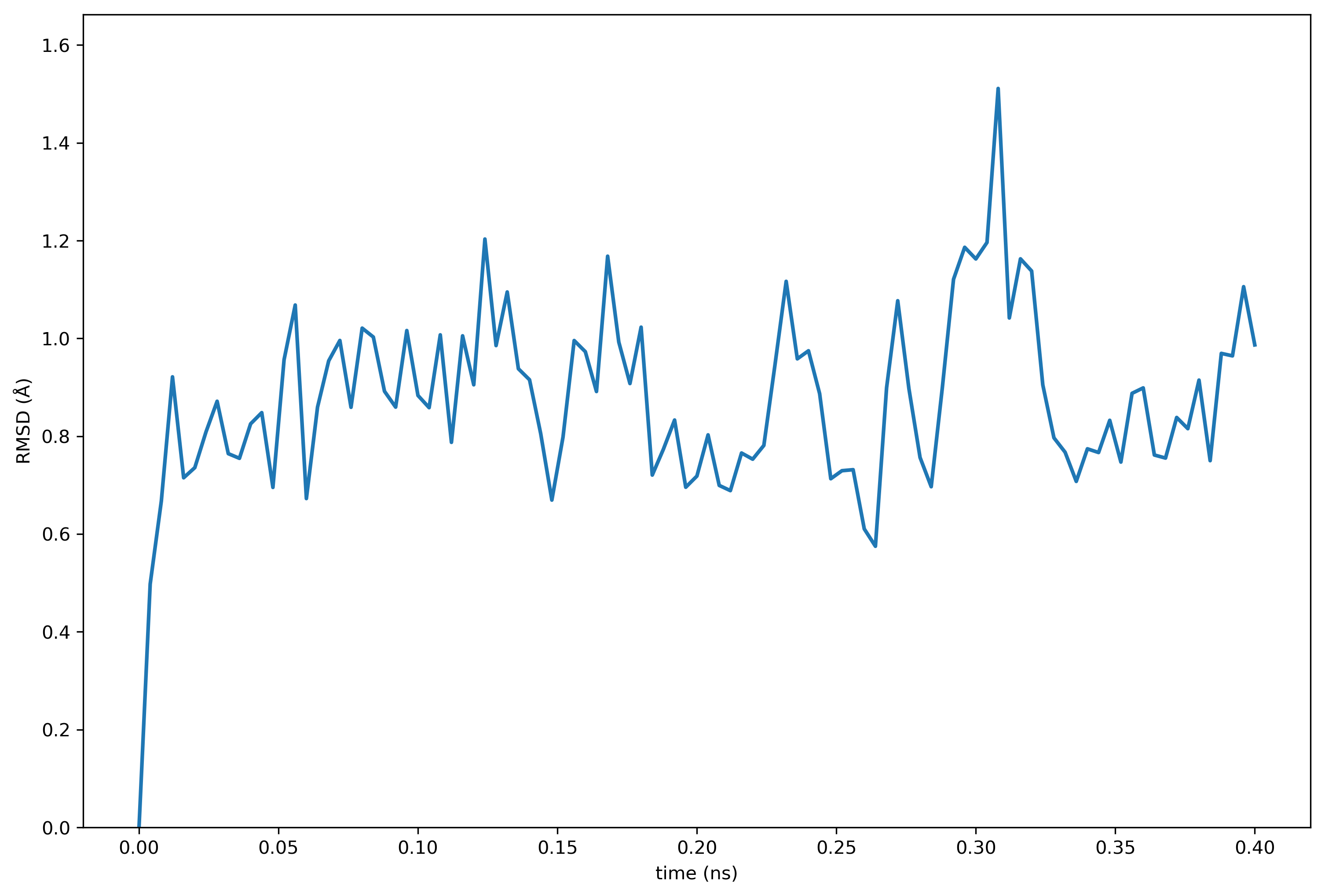
picturesave('fig.%s'%plotname,work.plotdir,
    backup=False,version=True,meta={})

You can generate the RMSD plot by running the following command.

make plot protein_rmsd

Omnicalc will deposit you in an interactive terminal in case you wish to inspect the data. Otherwise the following plot will be written to the plot_spot directory set in the connection file.

Note that this quickstart guide was tested and added to the validation list. The calculations repository has been shared according to the directions below, and can be found on github.

Sharing calculations

At the beginning of the quickstart guide we made a connection file which set the location of our calculations repository repo: calc/PROJECT_NAME/calcs. Note that PROJECT_NAME is replaced with the project name proteins. When you run make connect proteins, the factory makes a new, empty repository at factory/calc/proteins/calcs/ and runs git init there to create a new repository. You can use git commit to save changes to the calculation codes, for example protein_rmsd.py in this folder. To share the codes via github, you can make a new repository and then send your code there via git remote add origin https://github.com/username/my_repo and git push -u origin master. Other users who wish to use your calculations should set repo: https://github.com/username/my_repo in their connection files. When they run make connect new_project then the factory will clone the calculations repository from github to factory/calc/new_project/calcs so they can try your code. The calculations for the quickstart guide were shared on github using this method.

4. A web-based simulation-analysis pipeline

Pipeline documentation is available on a separate walkthrough.

5. Running the factory in Docker

The authors have tested the factory inside of Docker in order to (1) make sure that the code works, (2) serve the factory securely over a network, and (3) provide new users with the tools necessary to deploy the software on different platforms. Both dockerfiles and unit tests for the most important factory use-cases are provided on github and provide a lingua franca for setting up these codes. They are particularly useful when troubleshooting a software dependency problems.

Users who wish to test the code or serve a factory over the network should install docker first. See the docker installation guide for instructions. Docker will require root access to your machine. Users who only want a guide for setting up their software environment can simply read ahead for links to the dockerfiles and unit tests.

To test the factory, we will first clone it and connect it to extra tools designed to interact with docker. Note that this is somewhat counterintuitive: we create a factory for testing (hereafter factory-docker) which will later create a factory for deployment inside of a special root folder on your host. The testing factory will be small, and is only used to supervise the code. The deployed factory will be installed specifically for a docker container, and will be unusable on the host because the virtual environment sets a single root path when it is installed, and cannot be moved after installation.

The following commands can be used to create a testing factory.

git clone http://github.com/biophyscode/factory factory-docker
cd factory-docker
git clone http://github.com/bradleyrp/docks
git clone http://github.com/bradleyrp/factory-testset tests
make set commands mill/setup.py \
mill/shipping.py mill/factory.py docks/docks.py
# get VMD and Miniconda installers and set their locations
make set location_vmd_source ~/libs/vmd-1.9.1.bin.LINUXAMD64.opengl.tar
make set location_miniconda ~/libs/Miniconda3-latest-Linux-x86_64.sh
make set docks_config tests/docker.py
make set docks_testset_sources testset.py

This procedure downloads two critical files. First, tests/docker.py includes all of the dockerfiles. When we run a unit test, the code will automatically make docker images described in this file. There are multiple images depending on whether we need GROMACS, VMD, or ffmpeg for encoding videos. Second, tests/testset.py containts all of the unit tests and is designed to be self contained. Each test has instructions for writing files, creating a script composed of terminal commands, and even mounting a folder on your host inside of the docker. The unit tests are designed to be self-contained, and somewhat readable. Users who are interested in viewing either the dockerfiles or unit tests can find them at the following direct links.

1. Dockerfiles via docker.py
2. Unit tests via testset.py

To serve a factory from docker, you must first change the DOCKER_SPOT variable inside tests/testset.py. This is the root for all of the files that docker writes, and it will contain the deployed copy of the factory. Once you have prepared a location, run the following command.

make test factory setup

Note that the arguments factory test are a sequence of descriptors that can be arranged in any order. The unit tests in testset.py are named by these sequences. If you wish to serve a factory, you must first find the demo serve unit test in testset.py. This test contains a public dictionary for the network settings. Add your hostname to the hostname list, and choose the port and notebook_port. You must open these ports; this requires root access and depends on your operating system. Lastly, you should set a username and password in credentials. Once you have done this, you can serve the factory from inside the docker using the following command

make test demo serve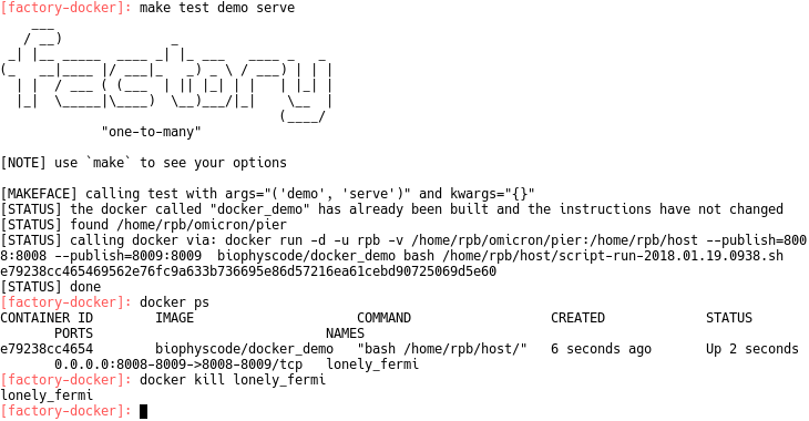

You can shut down the factory by running docker kill (see image above). The authors will provide more detailed documentation for the unit test syntax, however this guide has described the simplest way to test or deploy the factory. This quickstart guid is part of the validation list, and is necessary for running other unit tests. Contact the authors with questions!